Insert Data from Picture in Excel

An amazing feature is waiting for you on your Mobile Excel.

With the Insert data from picture feature that you will use on mobile devices like cell phone or tablet, you can get data to Excel from a picture.

Insert Data from Picture

Click the button on bottom left corner to view the Excel tabs.

You will see an image with a camera on it (Data from picture).

Click the Data from picture button and take a picture of your table.

After you take the picture, your data will be arranged in the background to be transmitted to Excel.

When the actions are complete, your table will be ready.


The action is as short and fast as that..

Azure PIM (Privileged Identity Management)

We can analyze the user roles on Azure under two different titles of Azure AD roles and Azure Resources roles as a platform. Microsoft has released the Azure AD Privileged Identity Management product for the management of these roles.

What can we do with the Azure AD Privileged Identity Management PIM product?

-You can assign privileged roles and define duration with the ticket or approval method for Azure AD or Resources.

– You can analyze all the action of the person who assigned or who got assigned by fetching activity logs through Azure AD Privileged Identity Management dashboard.

You need Azure AD Premium P2 or Office 365 E5 license to be able to use this product.


For Azure AD roles,

We can move on to the action steps.

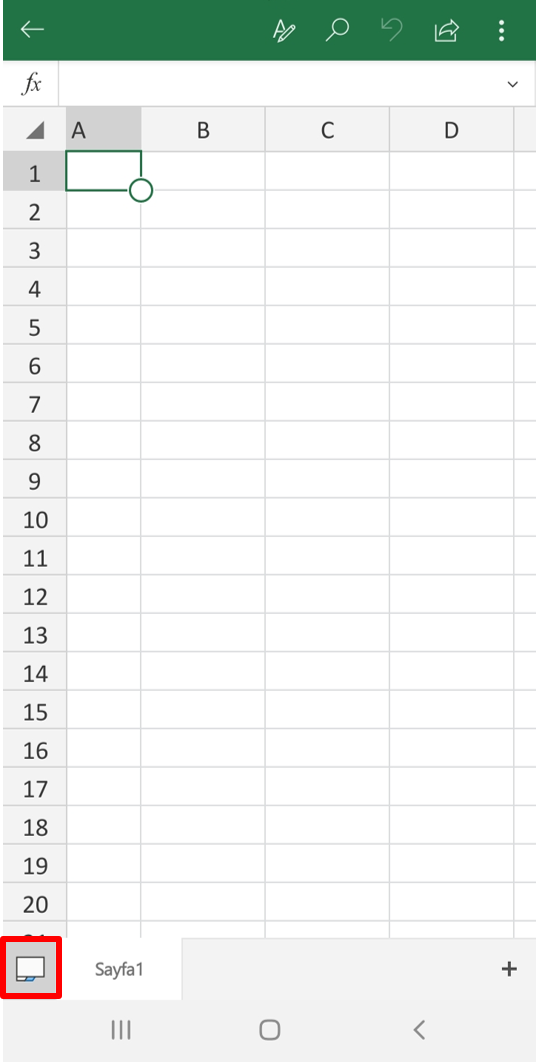
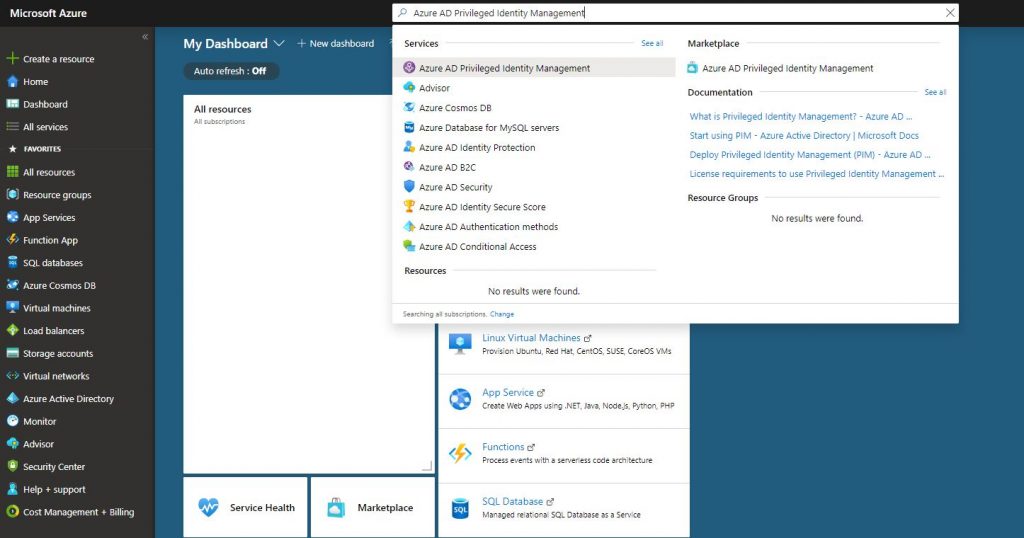
-Open the product by writing AD Priviliged Identity Management into the Search field on Portal Azure.

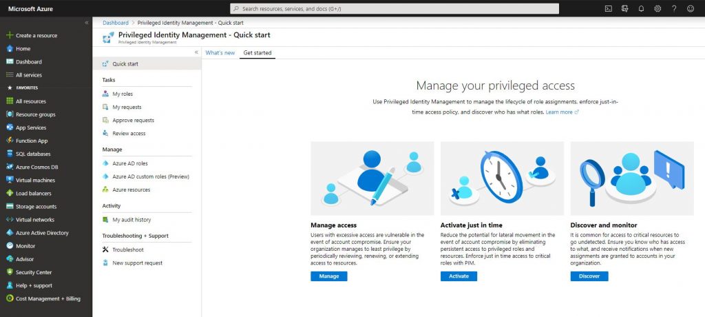
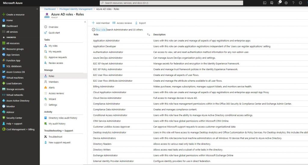
-A dashboard like the one below welcomes us when we open AD Privileged Management. We can do the necessary authorizations with the shortcuts on this dashboard.

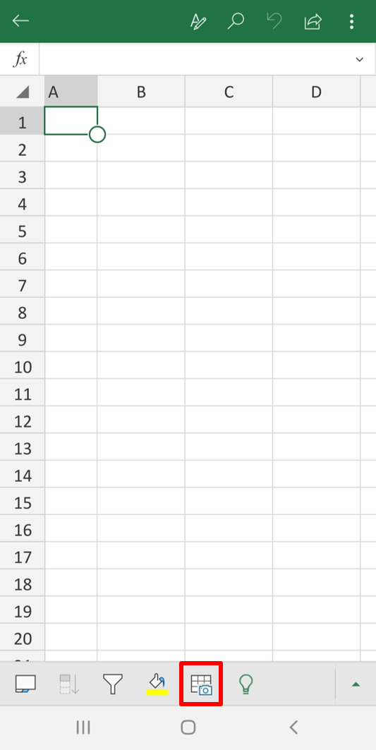
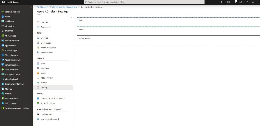
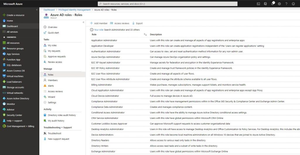
-After clicking Azure AD roles, go to settings and click roles.

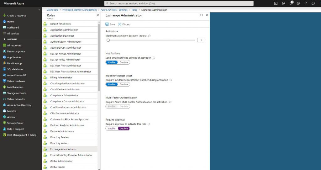
-Enable the Ticket in the field how the role will be active when it is assigned to the user.

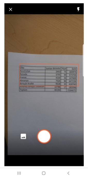
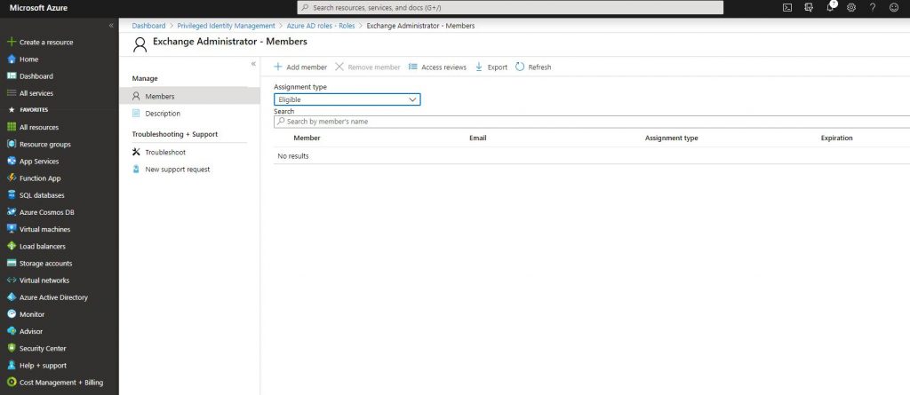
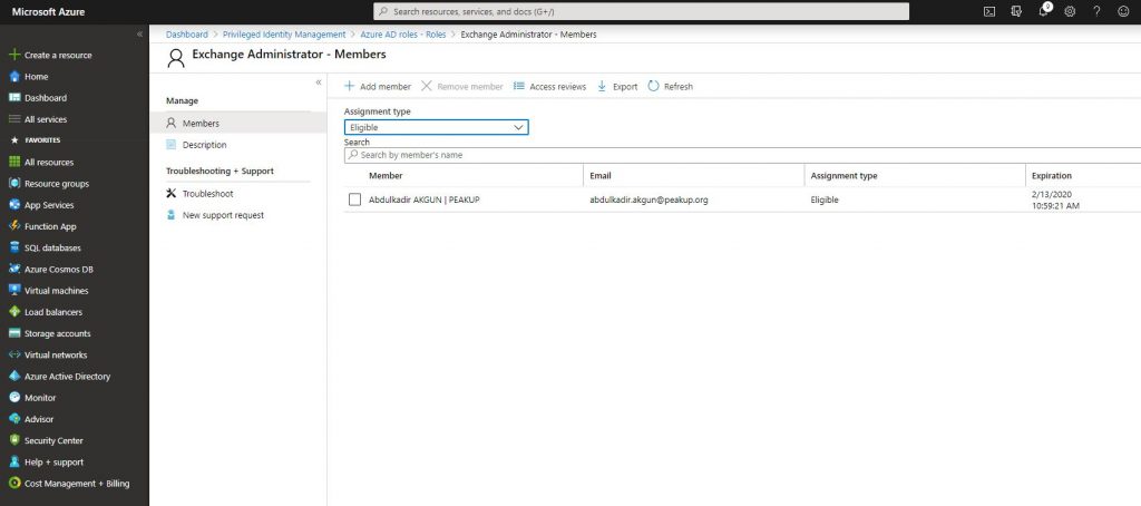
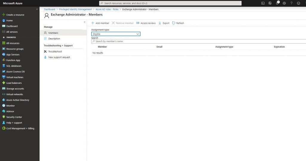
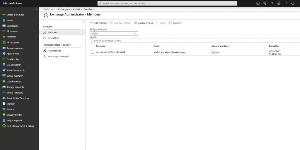
-Go back to the Azure AD Roles tab and go to Roles. Click Add Member and choose the user to whom you want to assign the role.

-Add the related user. The roles can be assigned as Eligible or Permanent. Since we will assign a role with a duration, choose Eligible.

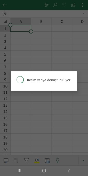
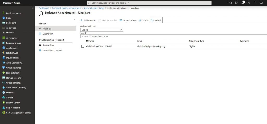
-We assign the role like you can see below.

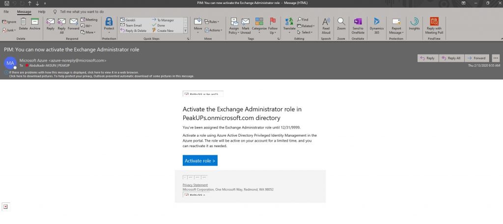
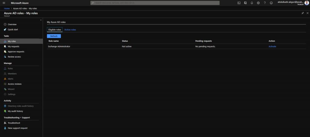
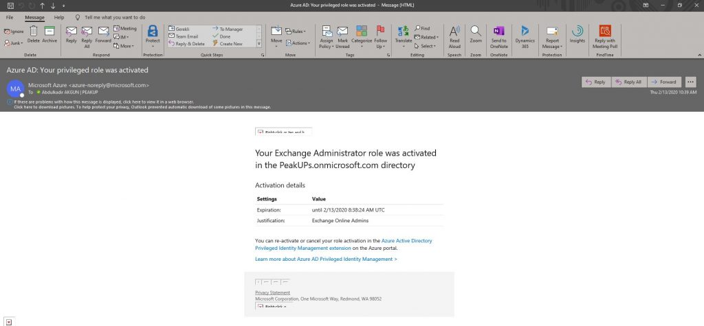
-A mail like the one below is send to the related user. Click the activate role button. You can access the related field by going to https://portal.azure.com with the user information and opening AD Privileged Management.

-Choose activate on the page that is opened.

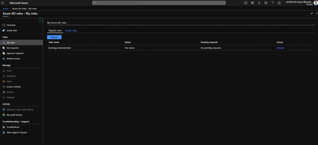
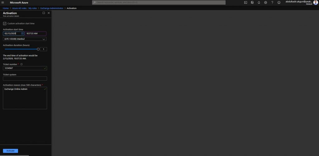
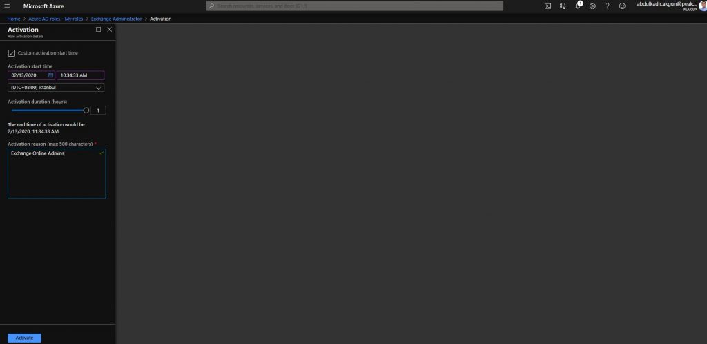
-You can specify a custom activation hour and have the role activated later. Ticket number and Activation reason fields are required fields and their content is optional. Write the content the admin or user have determined into the Ticker number field.

-After the activation action, the role has been activated like you can see below.

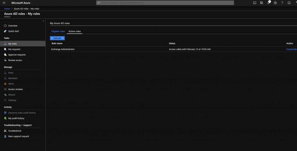
-You can see that the role has been activated and the expiration duration on the Azure AD Privileged Management dashboard.

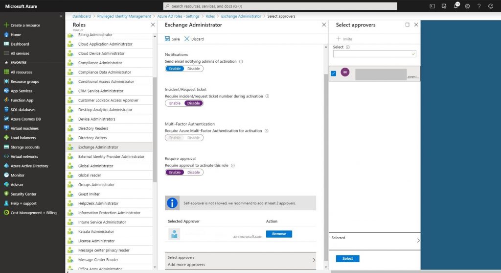
-Another role assigning method is the Require approval method. Let’s activate it in the related role like below. And choose the admin user that will approve.

-Open Manage-Roles.

-Choose Add Member and add the related user.

-Go to https://portal.azure.com with the related user and open AD Privileged Management. Click the Activate button.

-Write content optional to the Activation reason field. Click the activate button.

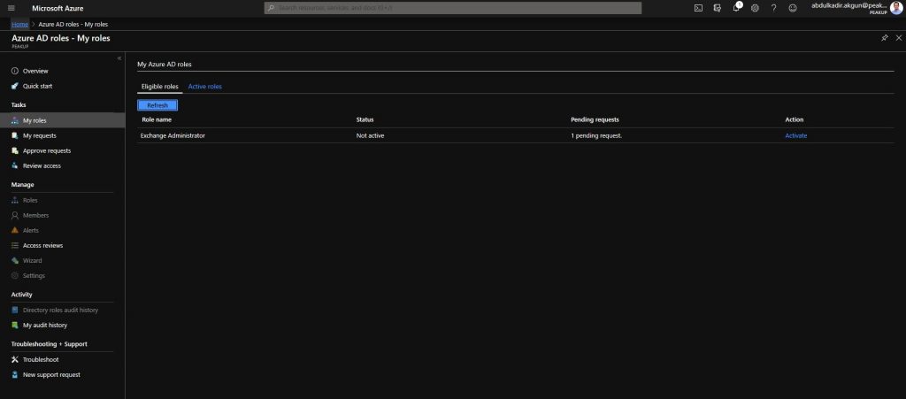
-The role will not be activated right away. Its status will be updated as pending request. A request will be sent to the Approver user we’ve stated in the role settings.

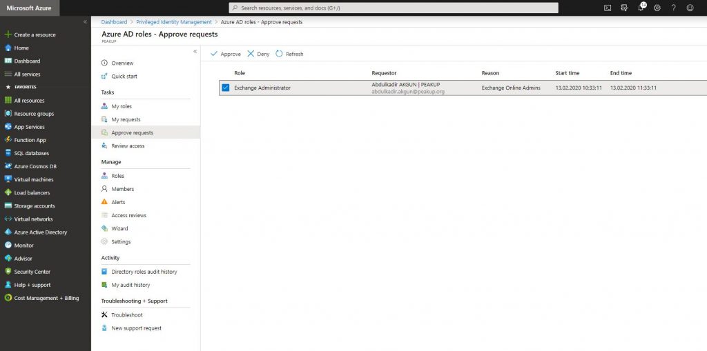
-Approver requests with the Approver user are seen like below.

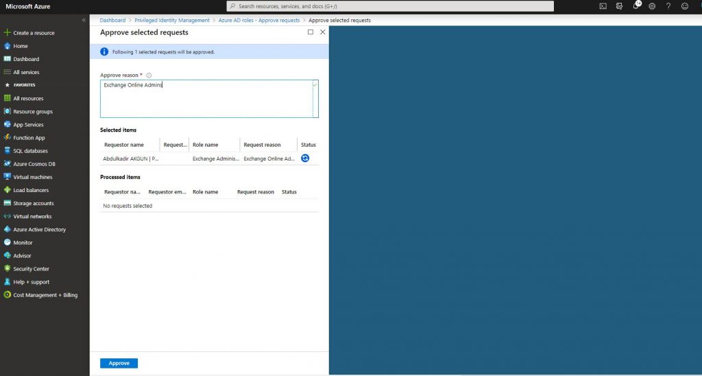
-After the request is approved, the role is activated.

-The related user is assigned to the role.

-A mail stating the the role is active will be sent to the user who we’ve assigned the role to.


For Azure resources,

-You can assign roles in Azure resources with Azure AD Privileged Identity Management. Open PIM through portal and click Azure resources. Then click Discover resources and add an available subscription.

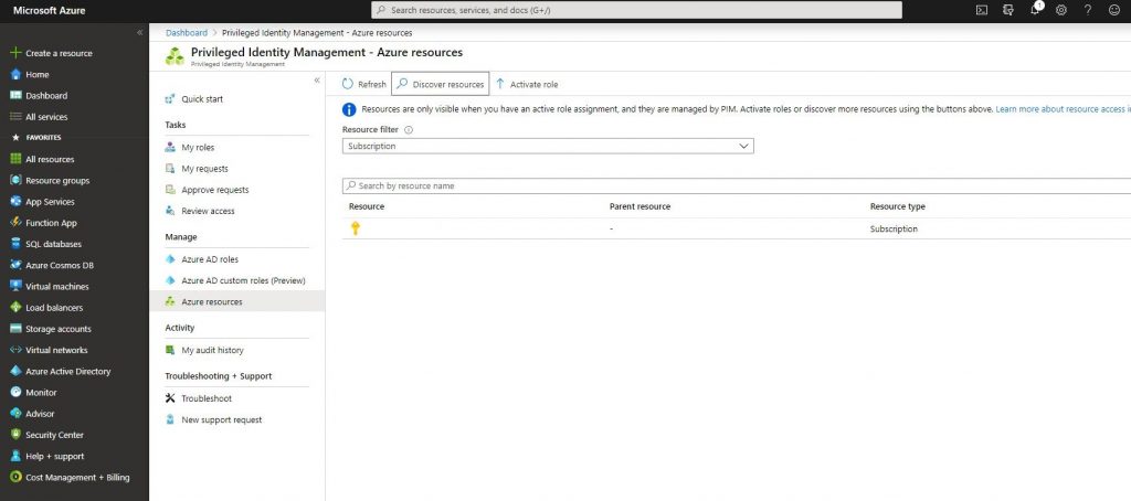
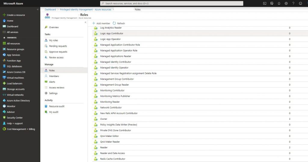
-Click the subscription you’ve added and go to settings like below. List your Azure resources roles. The steps from now on are the same as the ones with Azure AD roles.

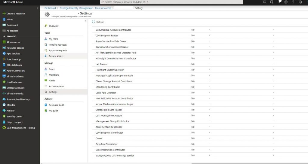
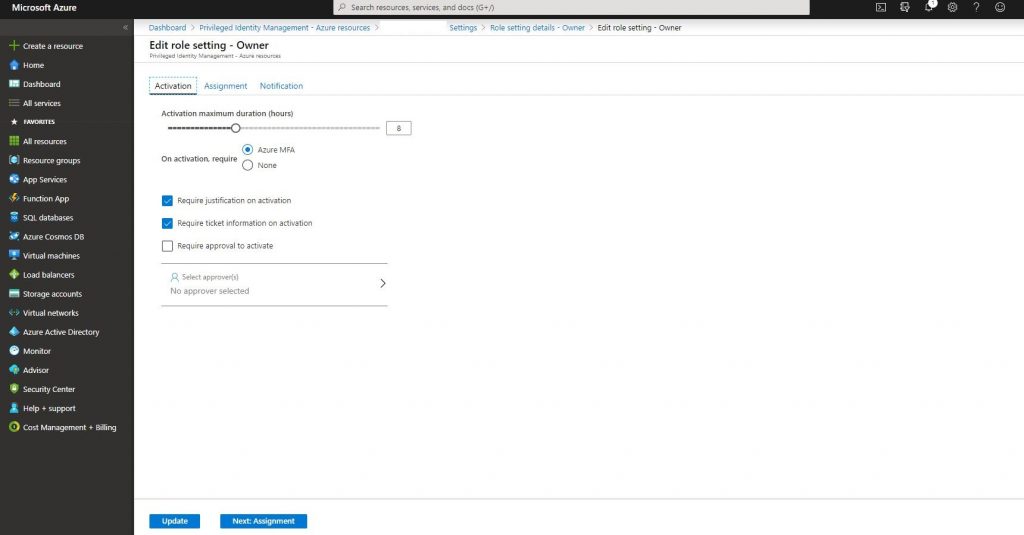
-Go into the owner role and click the edit botton.

-Determine if you will request MFA from the user who we will assign the role to before activating the role. You can take the same Ticket or Require approval actions as the Azure AD roles about how the role will be activated when it is assigned to the user.

-Go back to Azure resource and click roles.

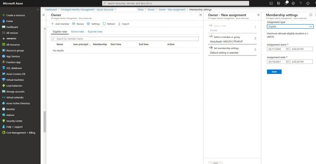
-Click add member and assign the role.

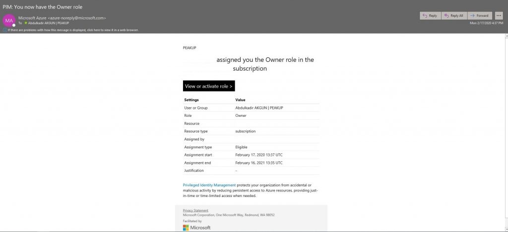
-You can activate with a Ticket or Approval like we did in Azure AD Roles steps. A mail like the one below is sent to the user. Click activate roles and complete the activation.

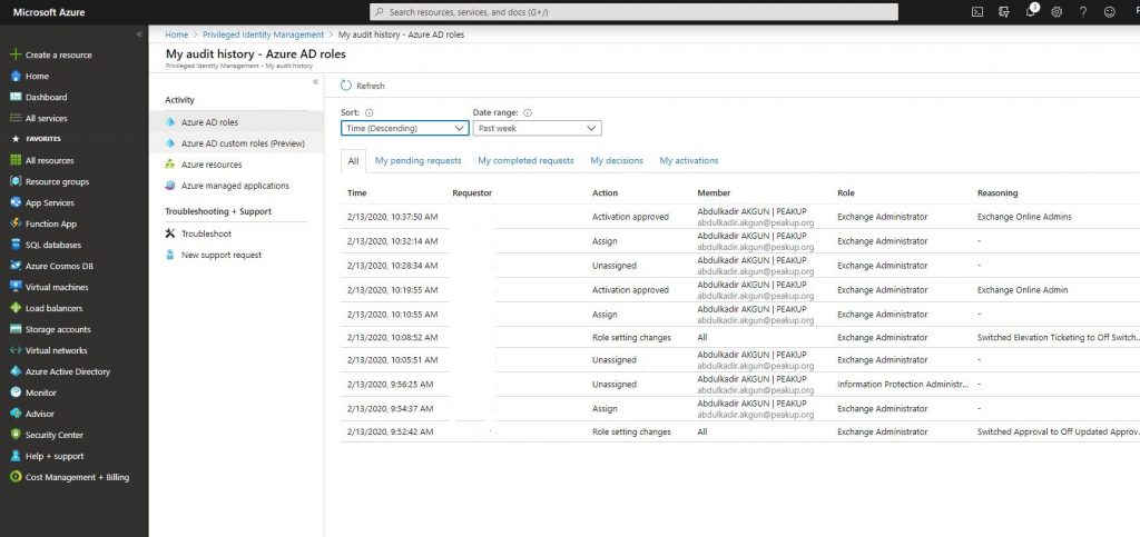
-We can analyze logs in My audit history for Azure AD Privileged Identity Management Azure AD Roles and Azure Resource.


Hope to see you later.


Page Redirect Actions

The Navigate function is used to switch between screens in PowerApps mobile applications.

How do you switch between pages?

By touching/clicking the items on the screen (with the user trigger)
Or automatically after a certain period of time (with a timer).

Usually the OnSelect property is used for all the actions that wanted to be executed the moment we “click”.

As an example, let’s take a look at how we switch to the next page when we click the next button on the page.

The page redirection action for the next button:

Navigate (target page, transition effect) will be written into the OnSelect property of this item.

You of course don’t have to write the Navigate formula to OnSelect all the time. We mentioned that different items have different properties. In this sense, properties like OnCheck, OnVisible, OnChange are used when necessary as well.

The OnCheck property can be used for a check box if you want it to work “the moment it is marked”.

CREATE A SPEEDOMETER CHART

SPEEDOMETER CHART


Hello everyone,

In this article, we will create a Speedometer chart. We will see how to create it simply step by step. Let me tell you this first: Microsoft will add this Speedometer chart to the standard charts for Office 365 users. I will be talking about the simplest version until then. I have stated what to do step by step below, please try to practice those steps with me. After learning how to create this chart, you can take a look at our Mouse Over Dashboard article. 😉


Let’s get started. 👍🏻


Before we start creating the chart, we have to have suitable data. We can create this chart with a few methods. We will use a combo chart in a data table to execute this action the shortest way possible.


⚫️ Let’s have this data starting from A1.

Indicator Index
25 0
35 2
40 100
100


⚫️ Choose any cell and click the Insert menu.

⚫️ Click Combo chart in the Charts group and then click Create Custom Combo Chart.

⚫️Choose the Chart Type of the Indicator as Doughnut on the Add Chart window that pops open. And choose the Chart Type of the Index as Pie and mark the Secondary Axis option, and then click OK.


⚫️ Click the + icon of the chart added to the page and unmark Chart Title and Legend.


⚫️ Right -click on the green area on the chart and then click Format Data Series. Make the Angle of the first slice 270 on the screen that opens up on right and press Enter.


⚫️ Go to Shape Fill in the Format menu and choose No Fill.


⚫️ Choose the Series “Indicator” option in the Current Selection field in the Format menu.


⚫️ Make the angle of the first slice 270 on the screen that pops open on right and then press Enter.


⚫️ We will remove the fill color of the purple piece at the bottom. For this press CTRL + (Right Key) 4 times and choose the purple Data Point and then go to Shape Fill in the Format menu and choose No Fill.


⚫️Now press CTRL + (Right Key) and choose the colors you want in the Shape Fill in the format menu for data points. If you want a bright image, you can use the Shape Effects. Note: If you click the same shape effect twice, it will become brighter.


⚫️ Choose the index only, right-click and add Data Labels. And then choose the data label and go to the formula bar, write equals to (=) and choose the B2 cell and press Enter. You can increase the font size of the data label and make it bold. The chart will look like this at this point.


⚫️If you want, you can add a Spin Button (Form Control) to the page that would make index move.

On the Developer tab, in the Controls group, click Insert, and then choose Form Controls and draw somewhere suitable in the page, for example to a blank area or a blank cell. Note: You can make the index bolder by increasing the number 2 that is indicated as the Index thickness in the cell B3.

⚫️ Right-click the form control item you’ve added and click Format Control. Go to Cell Link and choose the cell B2. And arrange the others values as the ones below.


⚫️Your Speedometer chart will be ready when you choose a circle among the Shapes and add into the middle of the chart.


Lastly, I want to share the file I have prepared with you.
You can download the file here. 👉🏻 

You can share this article and help many other people get informed as well.

Goodbye. 🙋🏻‍♂️

PowerPoint Shortcuts: The Most Frequently Used

You can have full control during your presentation with the PowerPoint shortcuts.

Start the Presentation: F5

You can start your presentation with the F5 shortcut.

Advance to the Next Slide: N

You can use the N key to advance to the next slide.

Return to the Previous Slide: P

You can use the P key to return to the previous slide.

You can use the N and P shortcuts (Next and Previous) to switch between slides.

Return to the First Slide: 1 + Enter

You might want to return to the first slide during the presentation. In this situation, you can return without having to return one-by-one. For that you need to press 1 and then Enter.

Start the Presentation from the Current Slide: Shift+ F5

You can start your presentation from the current slide without being lost between pages with the Shift F5 shortcut.

Display the Slide You Want: Slide Number + Enter

Use Slide page number and Enter to display the slide you want during the presentation. When you go 20 Enter you can go to the 20th slide.

Group Objects: Ctrl + G 

You can group the object for them to take actions together. Choose the object and then use the CTRL G shortcut for this action.

Blackboard: B 

You can use the screen as a blackboard during the presentation. You can write with a pen on the black background and make your presentation effective.

Whiteboard: W 

You can use the screen as a whiteboard during the presentation. You can write with a pen on the white background and make your presentation effective.

Erase all the Marks: E 

You can use this to erase all the marks done with the pen and cursor.

Return to the mouse cursor after you write with the pen: Ctrl + A 

You can use this shortcut to return to the mouse cursor after you write with the pen.

Hide the Pen or Cursor: Ctrl + H 

You can use this shortcut when you don’t want to see a pen or cursor in the screen.

Show hidden pen and cursors: Ctrl + U

Enables you to bring back the cursors you have hidden.

Save the Presentation As: F12

You can use this shortcut when you want to save your presentation as different formats like PDF or video, or when you want to change its location.

Now, you are ready you present faster with the PowerPoint shortcuts!

Shape Power Automate Flows Based On Forms Responses

We mentioned that it is possible to securely collect data in electronic environment with MS Forms. The automatic workflows are done with Power Automate flows.

In this article, we will create a flow that will be shaped based on the choices of the user by adding the Choose Action question.

If the user chooses Send Form to Approval, the Approval process is going to start. In the other case, only an info e-mail will be send.

After you add the Choose Action question to the Form, you can start the actions with a blank flow by switching to Power Automate.

Power Automate

While creating all flows, a trigger is created in the first step. Trigger is a required step for the flow to start working and it is important to specify it correctly. The flow we will create in this article will work when the Form is responded. So, the flow will be triggered every time the form is responded and will start to work. Add the When a new response is submitted trigger.  It is specified from the list of which poll is going to cause the flow to start when responded.

In the next step, we will look at the responses of the poll. Add the Get Response Details step to access the responses.

Choose the name of the poll in the Form Identity field. Choose Response Notifications List Response Identity for the Response Identity.

This step enabled us to access all question fields. This way, we can get the response of the Choose Action question.

In the new step, add Condition to test the response. Add the Choose Action question to the left with dynamic content.

And on the right, one of the responses will be written. Since we will be controlling a String, we will be using the String function.

It will be checked if the response given with the String(‘Send Form to Approval’) expression is equal to this value.

Add Approval to the Yes field of the Condition and Send an E-mail to the No field, and complete the process.

The approval mails can be sent to the person who has created the request (to the person who sent the form to approval) based on Approved/Denied condition.

Click here to read the other Power Automate articles.

THE TABLE FORMAT and ITS BENEFITS

In this article, we will be talking about the benefits of the table format of the data range in Excel. When we write titles and enter data under those title or when working on a prepared file we received, we say that we have prepared a table. But the data range we call a table is not a table for Excel yet. For it to be seen as a table, you need to format the data range as a table. At that point, it allows us to use a lot of features that table format allows us.

Now let’s take a look what we need to do before creating to table to use some features and how we do them after formatting as table. By the way, it would be very helpful to write the articles on our Blog when you have a chance. If you wish, you can read a detailed article on Office Support.


Choose Style for the Table Format

We can use this feature by choosing Format as Table in the Styles group in Home tab. Choose any cell on your data and click the Format as Table command and choose the table style you want. You will have turned your data into a table quickly. Don’t forget: Everything added to the page later is an object. An image, shape, chart, table, slicer etc. all of them are objects and a menu with features of objects added later is added to the Ribbon.

You can apply this feature easily with the shortcut keys.
Choose any cell on your data and turn your data into a table with the

  • CTRL + T

shortcut.


Now, let’s see what kind of features our data range gained with such a simple shortcut.


Benefits of the Table Format

  • When you choose a cell on the table and move upwards and downwards, the column titles will be the titles of your table. Thus, you don’t need to use the Freeze Top Row feature in the Freeze Panes field in the View tab.


  • A style is applied to our table automatically and each row is colored as dark and light successively one-by-one. And this creates a nice image.


  • When you keep entering data under the table or next to the table, your table gets longer and wider. And this enables the data we enter later to be included in the table and everything to be accepted as a whole.


  • Before applying the table format, when we want to get the 18% VAT in the Sum field written to the next column; we had to write the formula into a cell and drag it down first. If there are blank rows in between, we had do drag down again. But, when we format it as a table, it is enough to write the formula and press Enter for the formula to be applied on the whole column.


  • When we turn the data into a table, a menu named Table Design or just Design is created in the Ribbon. This menu contains the features that we can use for our table. One of the most important features is the Slicer feature that we are familiar with from the Pivot Table. This feature enables us to filter the area we want on our table with one click.


  • It allows us to add functions like sum, average, count, min, max easily when we filter on the table. You can take a look at the other Table Style Options.


  • When you create a Pivot Table from the data range, you have to choose Change Data Source most of the time when new data is added outside the field specified as the range. Considering that you add new data to your table every day, you will have to choose Change Data Source and specify the new data range all the time. But, when we turn our data into a table, the data we add under it or next to it will be accepted as a part of the table and is within the data range. Thus, it will be enough to Renew for the data to be reflected on the Pivot Table.


  • In the formulas, we get to specify the data range by writing the table’s name without having to choose the whole table.


We have seen a lot of positive features till now and we obtained them with CTRL + T only.

Big or small, we recommend you to use Format as Table while working with data.
This way, you will be able to use the features above that will make you gain visualization and speed.


Convert to Range

Lastly, when you want to convert your table to data range again, you have two options.

  1.  By choosing Convert to Range in the Table Design or Design menu.
  2. By right-clicking a cell on the table and choosing Convert to Range from Table.


I hope that this was a helpful article for you.
You can share this article with your friends and help a lot of people get informed as well.

Good bye. 👍🏻


Power BI & OneNote Relation: Publish to Web!

There is an increasing integration capacity among Microsoft products. We will start our article by talking about the integration between Power BI and OneNote. OneNote is a Microsoft product that has been released as a notebook and that has become more than a notebook with the updates it got. You can click here for general information about OneNote. You can get the text of an image with the updated (details here), and search between images (details here).

And Power BI is Microsoft’s popular reporting product. You can create interactive and impressive reports with Power BI. With the latest update, when you create a public Power BI report or come across one of those report and paste the report’s address to OneNote; OneNote automatically integrates with Power BI and show the interactive and live version of the report on itself. This way, it is not necessary for us to click the link and be directed to the website. And we don’t get to be left with the questions like which report was on this link.


Power BI bağlantısını OneNote'a kopyalama
Fig.1 – Copying the Power BI connection to OneNote

So, how do we make the reports made with Power BI public?

If you will not have any problems with sharing the reports you created with Power BI, you can make your reports public. After sharing, people don’t need to have Power BI license to view the report. It is enough for them to have the link.

Let’s take a look at how we create this link:

We will execute these actions on Power BI Web Portal ( app.powerbi.com). We don’t have to know with who and on which work environment this report will be shared in order to create the link. Open the report we want to share. Go to this option that was among “Export” options before through the “Embed” option on ellipsis. Click the “Publish to Web (Public)” command here.

publish to web komutuna erişim
Fig.2 – Access to the Publish to web command

You might come across two types of warning here:

1- Since this feature can be restricted on the Power BI Admin portal, it has to be enabled by your admin first. You might get an error message concerning this (Fig.3). If you get this error, you have to contact your admin and notify him/her.

Contact your admin to enable embed code creation
Fig.3 – Contact your admin to enable embed code creation

2- When you create this link, an info message indicating that this report and its content will be public and you shouldn’t use this feature is you will share it with certain people in the company will pop up (Fig.4).

Embed in a public website
Fig.4 –  Create an embed code for public reports that you can include on a website

Click the “Create embed code” option to share your report publicly. When you click, another warning message pops up(Fig.5). Click “Publish” as your last decision.

Embed in a public website
Fig.5 – Information about you are creating a code for public website

After you click, a link where we can share on mail, social media etc. and people can access is created. Right below it you will find the html format to embed it on a website (Fig.6). This way, anyone who has the link will be able to view this report doesn’t matter if they have license or not.

Link you can send in email
Fig.6 – Link of the code

When you have multiple embed codes or want to delete a link, you need to click on the setting icon and then click the manage Embed codes option in order to go to the window where you can manage these codes. You can get the embed codes again or remove these codes on the screen that pops up.

Manage Embed Codes
Fig.7 – Managing embed codes

Hope to see you in another article…

Good game well played.


CONCATENATE vs TEXTJOIN

CONCATENATE vs TEXTJOIN


Hello everybody!

In this article, I invite you to say goodbye to the old CONCATENATE function that when we wanted to add a space or any other character while concatenating the data, obliged us to do it one by one and thus that was very laboring, and say welcome to a more efficient function. If you need to join the data in multiple cells and add characters like a space, comma, semi colon, and hyphen; there is just one function that you need to use and that is the TEXTJOIN function.


WHAT DOES IT DO 

Like I mentioned above, you don’t need to click cells one by one and use an expression like ;” “; to add a space in between each time  or a statement like & ” ” & when joining with the & character in the textjoin function. It joins each cell in the selected cell range by adding the slicer we’ve indicated. This way, we can join the data in hundreds of cells easily as a text.


SYNTAX

TEXTJOIN(delimiter, ignore_empty, text1, [text2], …)

There are 3 main arguments in the function.

These 3 main arguments are required, the other arguments are optional.Now let’s take a look at what these arguments mean, i.e. what the function wants from us and what we will give it.


delimiter
(required)
A text string, either empty, or one or more characters enclosed by double quotes, or a reference to a valid text string. If a number is supplied, it will be treated as text.
ignore_empty
(required)
If TRUE, ignores empty cells.
text1
(required)
Text item to be joined. A text string, or array of strings, such as a range of cells.
[text2, …]
(optional)

Additional text items to be joined. There can be a maximum of 252 text arguments for the text items, including text1. Each can be a text string, or array of strings, such as a range of cells.


WORKING CONDITIONS

  • If the resulting string exceeds 32767 characters (cell limit), TEXTJOIN returns the #VALUE! error.
  • It came with Microsoft Excel 2019. If you are using and older Office version, you will get the #NAME? error and thus not be able to use this function.
  • If you Office 2019 or Office 365, you can easily use this function.


USING THE FUNCTION

After we write the function name, we specify the delimeter. And then we will choose how it should behave about the possible blank cells in the cell range. And in the last arguments, we choose the cell range to be joined. Now, let’s take a look at its use together.


In the example below, we join the data between the A and G columns with a semi colon in between them.


As you see, it is as easy as that to join a multiple cell range in a single text with any character between them.


See you in another articles, bye. 🙋🏻‍♂️
You can share this post with your friends and help them get informed as well.👍🏻

Briefing Concerning Covid-19 Pandemic for our Customers

]Corona Virus Covid-19 Pandemic Briefing and Emergency Action Plan

We have taken responsibility and brought a few practices to life in order to protect our employees, customers, suppliers and our shareholders because of Corona Covid-19 pandemic. You can download our emergency action plan to learn about the actions we take.