
What is Power Apps?
Power Apps is a product where you can develop customized mobile apps depending on your company’s needs.
What Can You Do with It?
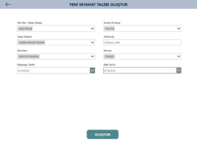
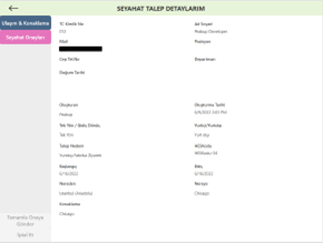
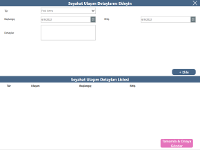
The processes of your company that are based on approval (Leave, Expenses, Advance, Company Vehicles etc.)
Management processes that need to be tracked (Contract Management, Library Management, Inventory Tracking etc.=
Stock tracking or product management systems (You can scan Barcodes, QR Codes, IMEI codes.)
The scenarios mentioned above any many other systems can be easily developed and used with Power Apps.
How Can I Use the Apps?
The apps you have developed with Power Apps work on all mobile devices (cell phone, tablet, computer).
You can download the Power Apps application on App Store, Play Store or Google Store for mobile devises and view and use all the mobile apps of your company under one roof.
And on computers, it is supported in all web browsers.
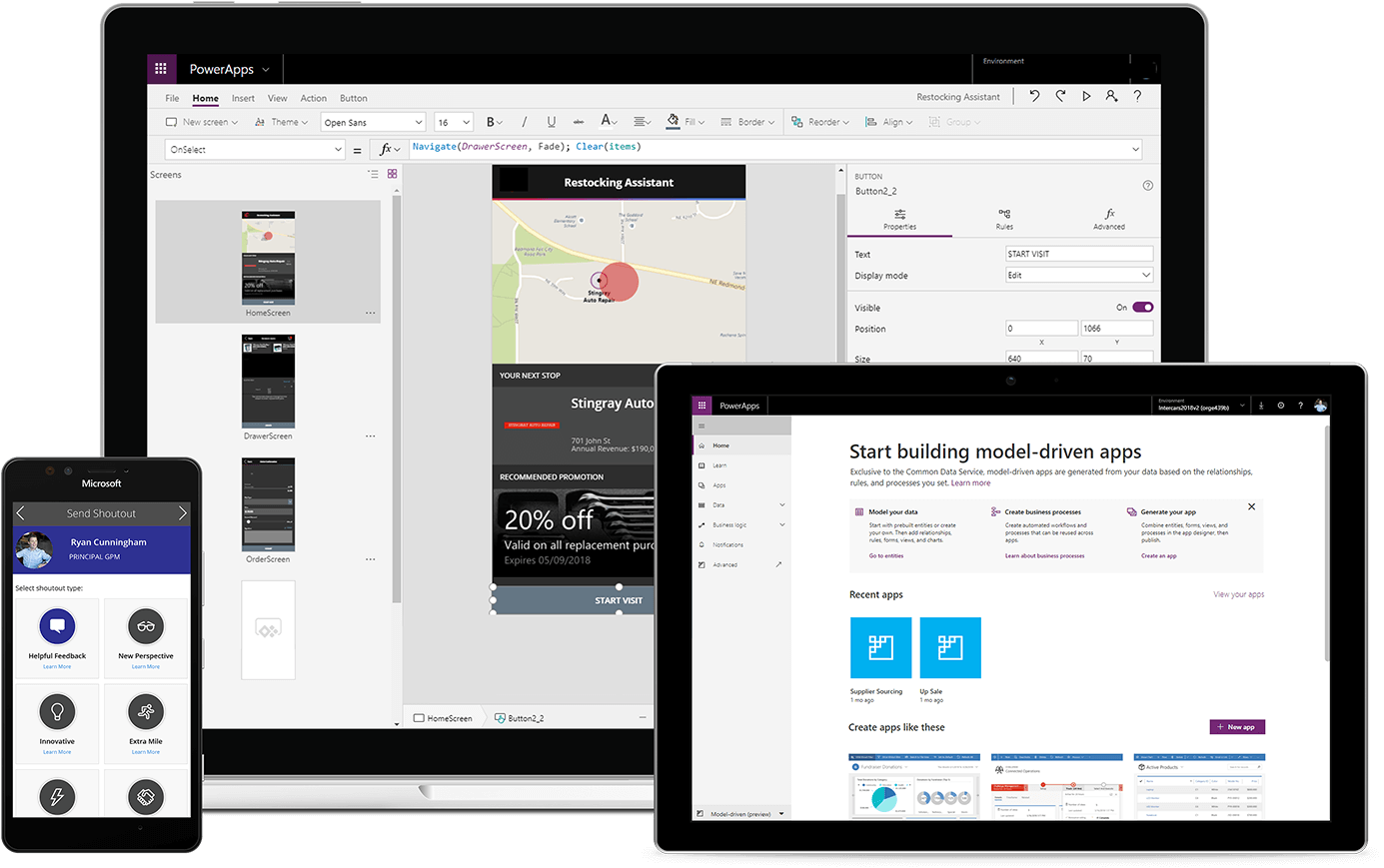
How Can I Develop an Application with Power Apps?
You can access the Developer interface (create.powerapps.com) through the desktop app or web browser and develop.
*Being able to develop apps through web browsers allows you to develop anywhere, anytime and with any device.
Do You Need to Be a Software Developer to Develop an App?
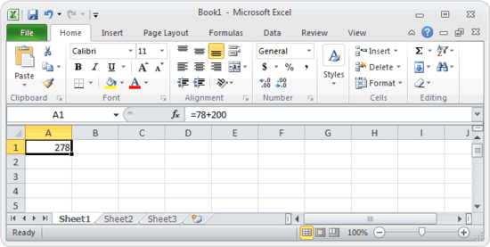
With the formula language you are familiar from Excel, it is very easy to code on Power Apps.
Power Apps has its own software language and its own functions. Alongside these functions, it also has a lot of functions (date, text, statistics etc.) that are available in Excel. Functions are in use in a general frame without being categorized.
You can manage an item on the screen of your mobile app easily by coding on the formula bar.
What Are the Skills of Power Apps?
- The app has integration with over 100 data sources.
- Getting, updating and deleting data are the most basic actions.
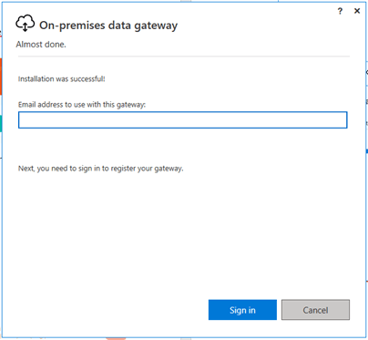
- You can use GateWay to access the data that are not on cloud.
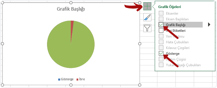
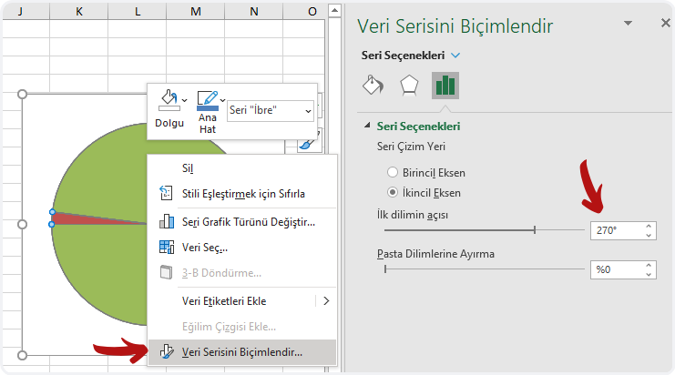
- The app interface is open to visualization and you can make visualization the way your imagination desires.
On the screens of your application:
- You can get warnings for user redirections.

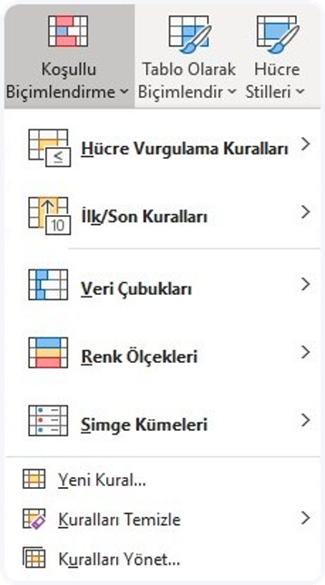
- You can use conditional formatting in the fields where data entry is obligatory and increase visualization and also verify data.
- You can inform the users instantly with mobile notifications.

- You can do many more things without any limits.