THE FILTER FUNCTION
Hello everybody,
In this article, will talk about the abilities of the FILTER function that is one of the New Dynamic Array functions. As you know, new changes have been coming into our lives with the Office 365. We can tell from the new Office apps updates and fixes published in the Office Insider Fast channel that Microsoft cares about developing Excel -its one of the strongest weapons- and that has focused on this product with Teams.
I mentioned in the XLOOKUP article that I was going to talk about the FILTER function details in its own article. Now, it is this function’s turn.
WHAT DOES IT DO?
Imagine creating Filters in one field or more. You can list all the record quickly without filtering the rest of the data on the screen with the FILTER function. For example: List me all the Murats in the A column. As you know, the VLOOKUP function gives us one result and brings the first data it finds, unfortunately doesn’t bring the others. The FILTER function brings us all the records. Now we can list the data as a whole with this function without using macros of writing array formulas. The use of the function is quite simple, keep reading for the details. 👍🏻
SYNTAX
=FILTER(array; include; [if_empty])
There are 3 arguments in the function.
The first 2 are required and the last one is optional.
Now let’s take a look at what these arguments mean, i.e. what the function wants from us and what we will give it.
| array
Required |
The array, or range to filter |
| include
Required |
A Boolean array whose height or width is the same as the array |
| [if_empty]
Optional |
The value to return i |
USE OF THE FUNCTION
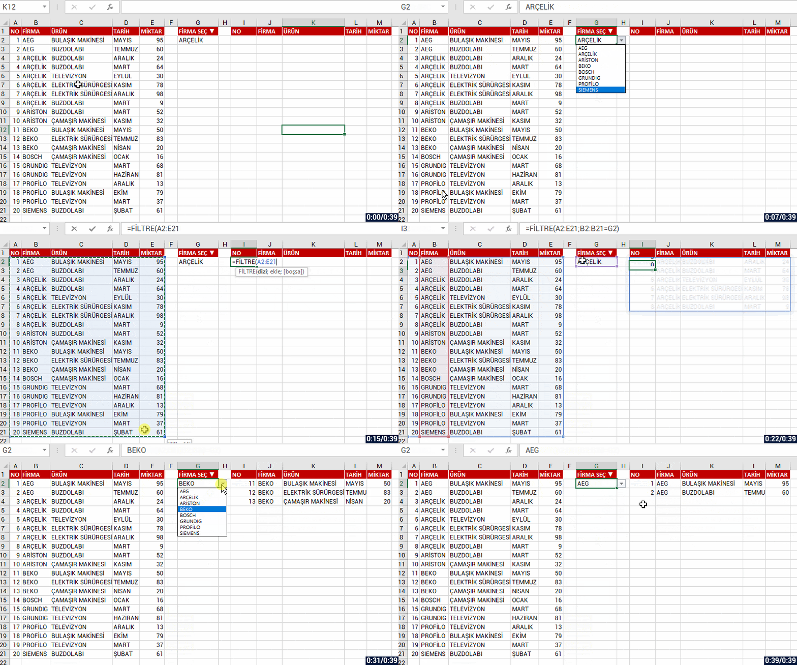
First, let’s list the data based on one criterion.
Let’s list based on FİRMA(COMPANY) and all the records of that company. Let’s choose bring the data of the company we choose from the FİRMA SEÇ(CHOOSE COMPANY) cell and if you like, let’s send a message like “No Record” if no data is found. For this, when you write no record into the [if_empty] argument; the text will be written into the cell if a data will not be returned.

USING MULTIPLE DYNAMIC CRITERIA
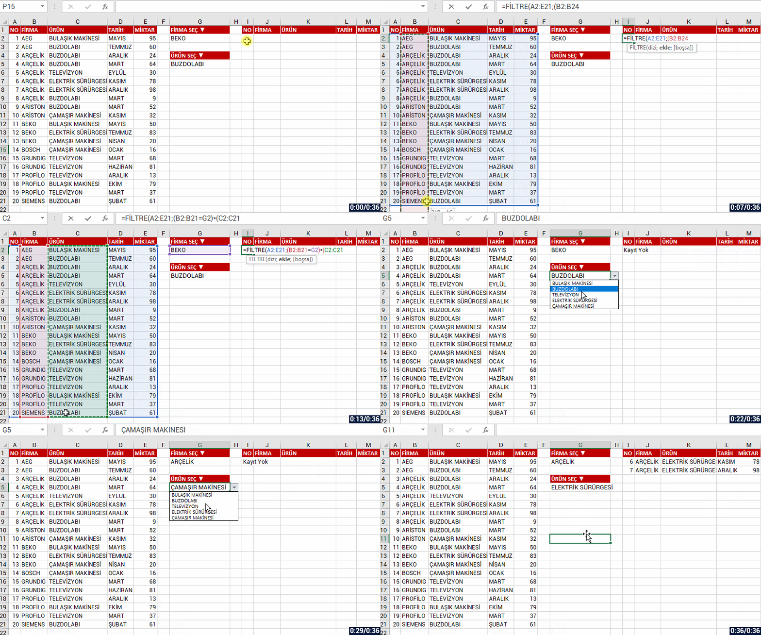
Into the insert argument of the function, we can list the results as a whole if there is data that match the criteria you’ve stated in multiple fields. For example, let’s have two criteria and list the data that match these criteria in the COMPANY and PRODUCT fields. For this, we write each of our criteria into parenthesis and add * (star/cross) in between the criteria.

We will be talking about the other New Dynamic Array functions in our next articles.
And then we will be able to get things done way easier by using these new functions together. I can’t help but wish that these formulas have had come out 15 years ago. 😀 LONG LIVE THE NEW DYNAMIC ARRAY FUNCTIONS!
See you in other articles, bye. 🙋🏻♂️
You can share this article and help a lot of people get informed as well. 👍🏻


