Microsoft Outlook Spaces

In this article, we will be giving information about Microsoft Outlook Spaces, which hasn’t been officially announced yet. It seems like Outlook is going to be the bomb! I think it is pretty assertive concerning the whiteboard look, drag and leave experience, viewing different apps in one screen. But there is a detail in the video that I want you to pay attention to: we can view multiple projects in different whiteboards.

Microsoft is working on Microsoft Outlook Spaces, which is a project management tool that unites all documents. The address is going to be: https://outlook.office.com/spaces but it is still under construction. WalkingCat -a famous Twitter account about leaks- have shared an online video concerning Outlook Space. If you want to follow this kind of leaks, you can follow WalkingCat on Twitter.
This new tool that can be accessed through Outlook web, makes it possible to organize and view different information of a certain project. It looks like a whiteboard where the user can pin different info from various Office 365 tools. I am already looking forward to Microsoft Outlook Spaces. 😎


Enabling Outlook Spaces


If you want to use Outlook Spaces right now, WalkingCat found a way to enable it a little early. You simply have to open up outlook.office.com/spaces and go into the developer tools on your browser (press F12). From there, go to the Console tab on the developer tools, copy and paste the following code into the console, and hit enter:

localStorage.setItem("featureOverrides", "outlookSpaces-enabled")

After that, refresh your browser and you’ll be allowed to get started with Outlook Spaces by creating your first project:


If you want, you can try it by following the steps below.

  1. Go to Https://outlook.office.com/spaces
  2. Open DevTools-> Application-> Storage-> LocalStorage on your web browse
  3. Add item: “featureOverrides“, value: “outlookSpaces-enabled”
  4. Refresh web browser


You can find other up-to-date articles on our blog.
You can share this post with your friends and get them informed as well. 👍🏻

SELECT CASE DECISION STRUCTURE

In this article, I wanted to share some information about the Select Case Decision Structure which is one of the Decision (Condition) Structures in Excel & VBA, a.k.a Excel macros. You can find other articles about Excel & VBA on our blog.


WHAT IS THE SELECT CASE DECISION STRUCTURE?

The Select Case Decision Structure

can be used to control comparisons about a data, just like the IF structure.
The values it returns are going to be True or False. When it is True, the code lines under it work. When it is False, if there are other Case conditions, they are controlled.
If there are other Case conditions and they are True, the codes below them are applied.
If there is no other Case conditions or all the Case conditions have returned False, if there are other codes in the procedure, they are applied by getting out the block with End Select.

Even though it is similar to IF (IF Else ElseIf Then) its type is a bit different and if you have multiple conditions, it is way easier to use compared to IF.


Here is the Syntax..

Blue

parts cannot be changed.
Red parts can be changed.
Green parts are comment lines.

Select Case Data to be controlled
‘Your Codes
End Select

If we are going to have multiple conditions, than Case Is or Case statements come into the play. We also have the Case Else statement that allows us to say “do this if the controlled data is outside indicated conditions.”

Select Case Data to be controlled
Case Is Condition
‘Your codes
Case Is Condition
‘Your codes
Case Is Condition
‘Your codes
Case Else
‘Your codes
End Select

If you want, you can write to codes in the same row after the condition part with : (colon). Case Is Condition: Your Codes
If we use a comparison operator (<; <=; =; >; >=) while indicating a condition, Case Is statement is written for the condition. If not, Case statement will be enough. You will see this situation in the examples below.

We used this statement for the Select Case structure above: “If you have multiple conditions, it is way easier to use compared to IF.”
Let’s give an example of this. We will apply the same conditions with both the IF structure and the Select Case structure and see the difference.
Our conditions will be like this: we have a value and we’ll have it checked. If this value is smaller than 1, we will return the outcome with MsgBox. Likewise, if it is between 1 and 5 or 6 and 10 or 11 and 15, we’ll return the outcome with MsgBox. We will prepare this separately with both of the structures.


Let’s start. First, the codes that we will need if we write our codes depending on the conditions above with the IF structure are:

Sub IF_Yapisi_ile_1()
For i = 1 To 10
If Cells(i, 1).Value < 1 Then
MsgBox "Değer 1'den küçüktür."
ElseIf Cells(i, 1).Value >= 1 And Cells(i, 1).Value <= 5 Then
MsgBox "Değer 1 ile 5 arasındadır."
ElseIf Cells(i, 1).Value >= 6 And Cells(i, 1).Value <= 10 Then
MsgBox "Değer 6 ile 10 arasındadır."
ElseIf Cells(i, 1).Value >= 11 And Cells(i, 1).Value <= 15 Then
MsgBox "Değer 11 ile 15 arasındadır."
End If
Next i
End Sub


If we want to write our codes in different IF rows for each condition and simplify it, then we can write it like this:

Sub IF_Yapisi_ile_2()
For i = 1 To 10
If Cells(i, 1).Value < 1 Then MsgBox "Değer 1'den küçüktür."
If Cells(i, 1).Value >= 1 And Cells(i, 1).Value <= 5 Then MsgBox "Değer 1 ile 5 arasındadır."
If Cells(i, 1).Value >= 6 And Cells(i, 1).Value <= 10 Then MsgBox "Değer 6 ile 10 arasındadır."
If Cells(i, 1).Value >= 11 And Cells(i, 1).Value <= 15 Then MsgBox "Değer 11 ile 15 arasındadır."
Next i
End Sub


Now let’s see how we will write the same conditions with the Select Case statement.

Sub Select_Case_Yapisi_ile()
For i = 1 To 10
Select Case Cells(i, 1).Value
Case Is < 1: MsgBox "Değer 1'den küçüktür."
Case 1 To 5: MsgBox "Değer 1 ile 5 arasındadır."
Case 6 To 10: MsgBox "Değer 6 ile 10 arasındadır."
Case 11 To 15: MsgBox "Değer 11 ile 15 arasındadır."
Case Else: MsgBox "Değer 15'den daha büyüktür."
End Select
Next i
End Sub


We saw that we can execute the action we want with three different codes and we can increase this number, but I hope that you can see the difference between them.
With the IF structure, we had to indicate Cells(i, 1).Value –the cell address that we were going to have controlled and we wrote it many times to indicate the condition between two numbers. But with Select Case, it was enough for us to write the cell address that we were going to have controlled and it was very easy to indicate the condition between two numbers as 1 To 5.

Let’s see the outcome with the Select Case structure in a GIF.

select case karar yapısı vba


CODE SAMPLES

You can apply the Select Case application samples below and test how it works and comprehend its logic better.

Sub Makro1()
Select Case "Murat" = "Emre"
Case True: MsgBox "İfade Doğrudur."
Case False: MsgBox "İfade Yanlıştır."
End Select
End Sub


Sub Makro2()
Dim Değer As Integer
Değer = 2
Select Case Değer
Case 1: MsgBox "Değer 1'dir."
Case 2: MsgBox "Değer 2'dir."
Case 3: MsgBox "Değer 3'tür."
Case Else: MsgBox "Değer Mevcut Değil."
End Select
End Sub


Sub Makro3()
Dim Değer As Integer
Değer = 1
Select Case Değer
Case Is < 1: MsgBox "Değer Küçüktür."
Case Is = 1: MsgBox "Değer Eşittir."
Case Is > 1: MsgBox "Değer Büyüktür."
End Select
End Sub


Sub Makro4()
Dim Metin As String
Metin = "PEAKUP"
Select Case Metin
Case "Excel": MsgBox "Metin Excel'dir"
Case "PEAKUP": MsgBox "Metin PEAKUP'tır."
Case "VBA": MsgBox "Metin VBA'dır."
End Select
End Sub


Sub Makro5()
Dim Değer As Integer
Değer = 14
Select Case Değer
Case Is < 1: MsgBox "Değer 1'den küçüktür."
Case 1, 2, 3, 4, 5: MsgBox "Değer 1 ile 5 arasındadır."
Case 6, 7, 8, 9, 10: MsgBox "Değer 6 ile 10 arasındadır."
Case 11, 12, 13, 14, 15: MsgBox "Değer 11 ile 15 arasındadır."
Case Else: MsgBox "Değer 15'den daha büyüktür."
End Select
End Sub


Sub Makro6()
Dim Değer As Integer
Değer = 20
Select Case Değer
Case Is < 1: MsgBox "Değer 1'den küçüktür."
Case 1 To 9: MsgBox "Değer 1 ile 9 arasındadır."
Case 10 To 19: MsgBox "Değer 10 ile 19 arasındadır."
Case 20 To 29: MsgBox "Değer 20 ile 29 arasındadır."
Case Else: MsgBox "Değer 29'dan büyüktür."
End Select
End Sub


Sub Makro7()
Dim Değer As Long
Değer = 15
Select Case Değer
Case Is < 1: MsgBox "Değer 1'den küçüktür."
Case 1 To 4, 5 To 9: MsgBox "Değer 1 ile 9 arasındadır."
Case 10 To 14, 15 To 19: MsgBox "Değer 10 ile 19 arasındadır."
Case 20 To 24, 25 To 29: MsgBox "Değer 20 ile 29 arasındadır."
Case Else: MsgBox "Değer 29'dan büyüktür."
End Select
End Sub


Sub Makro8()
Dim Tanım As String
Tanım = "C"
Select Case Tanım
Case Is < "E": MsgBox Tanım & " harfi E harfinden önce gelir."
Case Is > "E": MsgBox Tanım & " harfi E harfinden sonra gelir."
End Select
End Sub


Sub Makro9()
Dim Tanım As String
Tanım = "E"
Select Case Tanım
Case "A" To "M": MsgBox Tanım & " harfi A ile M harfleri arasındadır."
Case "N" To "Z": MsgBox Tanım & " harfi N ile Z harfleri arasındadır"
Case Else: MsgBox "Case Else"
End Select
End Sub


You can cat more detailed information about the Select Case statement on Microsoft Docs.


See you in other articles, bye. 🙋🏻‍♂️
You can share this post with your friends and help them get informed as well.👍🏻

The RANDARRAY Function

In this article, I will be talking about one of the new dynamic array functions: the RANDARRAY function. Sometimes we need a data table filled out with random data. With this function, you can quickly fill as many rows and columns with numeral data. And you can find our articles about other functions on our blog.

WHAT DOES IT DO

The RANDARRAY function returns an array of random numbers. You can specify the number of rows and columns to fill, minimum and maximum values, and whether to return whole numbers or decimal values. The function returns a random set of values between 0 and 1 if you don’t enter an argument. For example, you can create a 20-row and 5-column table that contains whole numbers between 50 and 500 quickly in a few seconds.You will see an example below.

SYNTAX

=RANDARRAY([rows],[columns],[min],[max],[whole_number])This function has 5 arguments.
All of them are optional.

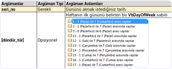
Now, let’s take a look at these arguments and what they mean, and what we will give them.
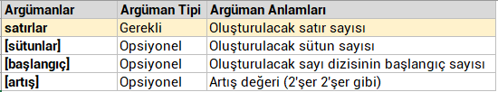
[rows]

Optional

The number of rows to be returned
[columns]

Optional

The number of columns to be returned
[min]

Optional

The minimum number you would like returned
[max]

Optional

The maximum number you would like returned
[whole_number]

Optional

Return a whole number or a decimal value

  • TRUE for a whole number
  • FALSE for a decimal number.


WORKING CONDITIONS

  • If you don’t input a row or column argument, RANDARRAY will return a single value between 0 and 1.

  • If you don’t input a minimum or maximum value argument, RANDARRAY will default to 0 and 1 respectively.
  • The minimum number argument must be less than the maximum number, otherwise RANDARRAY will return a #VALUE! error.

  • If you don’t input a whole_number argument, RANDARRY will default to FALSE, or decimal value.
  • The RANDARRAY function will return an array, which will spill if it’s the final result of a formula. This means that Excel will dynamically create the appropriate sized array range when you press ENTER. If your supporting data is in an Excel table, then the array will automatically resize as you add or remove data from your array range if you’re using structured references. For more details, see this article on spilled array behavior.

  • RANDARRAY is different from the RANDfunction in that RAND does not return an array, so RAND would need to be copied to the entire range.
  • An array can be thought of as a row of values, a column of values, or a combination of rows and columns of values. In the example above, the array for our RANDARRAY formula is range D2:F6,or 5 rows by 3 columns.
  • Excel has limited support for dynamic arrays between workbooks, and this scenario is only supported when both workbooks are open. If you close the source workbook, any linked dynamic array formulas will return a #REF! error when they are refreshed.


USE OF THE FUNCTION

Now, let’s see how this function works with 3 different examples. First, we will determine rows and columns. And then we will give row, column, min and max number values and return a retrospective array. And then, we will request the numbers to be returned to be whole number. The image we will obtain is going be like this:


excel rasgdizi farklı örnekler


See you in other articles, bye. 🙋🏻‍♂️
You can share this post with your friends and get them informed as well. 👍🏻


Power BI : 2020 March Favorites

Hello, here we are with the Power BI March update! I realize how fast the months go by with the new updates. This month, we have some long-waited and nice updates. In this sense, Power BI users’ opinions were taken into consideration. If you have all buckled up, let’s start!


1- New Action Alert

The most eye-catching feature in the Power BI March updates! New action options are available for the buttons we add for more interaction and a better application image:

  • Page Navigation
  • Drill through

We tried to find our way with the Page Navigation action to this day: by adding a bookmark with the most unfiltered version of the other page. Microsoft found out that we solved it like the and stepped in and offered this as an action option to do this the legal way. I can spend all my applause on this feature.


page navigation
Page navigation


The second one is one of the actions we wanted to see in the scenes. We were so happy about even the “Right-click to use the drill through.” text! -Because normally we had to go to charts and right-click to find that feature!- That’s why we are extremely happy about it.

tablo detayını gör
Activating the Drill through feature through the “See table details” button.


When we choose the Drill through as action, we can print the chosen one with conditional formatting and this helps a lot in terms of having an image that puts people into action. Also, you can write tooltip texts  for when its active/passive.

Koşullu Biçimlendirme&Enabled Tooltip
You can print the selected value by using conditional formatting for the text in the button and make it visible by writing any text you want to the Enabled Tooltip area.


Disabled Tooltip
You can write what you want to do into the tooltip field in order to activate the button.

2-Multi-column sort for tables

Feels like it was just yesterday that you were crying “But why? We need this feature!” and I was saying “I know, I know, it is so ridiculous but it is what it is!” And now we finally got this update! To add more columns to the sort order, Shift + click the column header you would like to add next in the sort order.

birden çok sütuna göre sıralama
When you click a column title with the SHIFT key, it accepts that column as sorting measure as well.

3- Dual axis for line chart

It was our subjects in recent trainings! Now we can add a second axis that allows us to draw two trends with different ranges along the same X-axis progression. We can compare two different units in the same graphic at the same time. Like Sales Amount&Sales Total, Sales Tex&Sales Total…

4-Filter Pane Search

It was a feature that was available in web but not in desktop. Now it is available for desktop too. You can search the filter you want in the search area. This features is activates as default. You can turn this feature on or off in the reports settings of the Options dialog.

Filtrelerde arama

5-Updates to decomposition tree

Some people were very happy when the decomposition tree came us default to Power BI! The decomposition tree now supports modifying the maximum bars shown per level. The default is 10 and users can select values between 3-30. Setting a low number is particularly handy if you don’t want the decomposition tree to take up too much space on the canvas. That way it’s more useful.

ayrışma ağacının yeni özelliği

6-New DAX function: COALESCE

A new DAX Function enters our lives with the Power BI March updates. The COALESCE function returns the first expression that does not evaluate to BLANK. So, what the hell does this mean? There are already a lot of functions as “That does not evaluate to BLANK”… They syntax of this function is:

COALESCE(, [, ]…)


It goes like that step by step and shows us the non-blank one. As outcome, it returns us a scalar expression. We can use it in an example like that:

When we do a calculated and show in on card, we don’t want the blank expressions to be visible. We want something like 0,1,100,”-“. For this we use the IF(ISBLANK(…) expression. Right at this point we can use this function.

COALESCE (SUM (FactInternetSales [SalesAmount]), 0) = IF(ISBLANK(SUM (FactInternetSales [SalesAmount])),0)

7-Relations get stronger with ArcGIS!

Product of Esri -the most known map and cartography company of the world: ArcGIS. We have been using its maps as default anyways for a long time and knew that more detailed features would come. Most features are available for Premium and some can be used in Pro. First of all, let me show you the location of ArcGIS maps.

ArcGIS
ArcGIS location

When you click here, there are 3 types of connections:

  • ArcGIS Enterprise
  • ArcGIS Online
  • Standart


The ArcGIS Enterprise and ArcGIS Online options are for users who have the premium app subscription and provides all the capabilities of Standard and extra capabilities, including additional geocoding, technical support, and access to mapping reference layers, and more. The Standard option is free and provides basic mapping capabilities. I leave the features below for you to check them.

arcgis maps capacity&preferences

Multiple Reference Layer

All premium app users can now add multiple reference layers to a single map visualization within Power BI. A reference layer is information represented on a map. It adds context to your operational business data. For example, let’s say you have mapped your store locations in Power BI. You can now overlay it against reference layers such as income, age, competitor locations or other demographics to gain valuable insights. You can add data and layers that are published and shared online by the ArcGIS community as well as layers from your ArcGIS Online or ArcGIS Enterprise organization.

New table of contents

A new table of contents that will help all ArcGIS Maps for Power BI users (free and premium) better visualize their data on a map has been added. Now, when you drag data to a location field well and see it on a map, you can also see a table of contents that lists all the layers on the map and shows the features represented by the layers. This allows your report viewers to quickly understand the data that they are seeing.

arcgis_map

8-Data Sources

Is an update without a new data source an update at all?

  • HIVE LLAP: This connector provides both Import and Direct Query capabilities and the ability to specify Thrift Transport Protocol as ‘Standard’ or ‘HTTP’.
  • Cognite:  The Cognite Power BI connector enables data consumers to read, analyze, and present data from Cognite Data Fusion (CDF).

We have shared our favorite updates for this month. You can click here for our other articles about Power BI. Click here to download the latest version of Power BI Desktop.

Good game well played.


MASS E-MAIL WITH EXCEL THROUGH OUTLOOK

In this article, I will be talking about how we can execute an action which I know that many users need in Excel Training. Without further ado, let’s see how we can send a mass e-mail with Excel through Outlook.

excel toplu mail

First of all, we will be sending mass e-mails with Excel through Outlook with the power of VBA, a.k.a macros. So, it wouldn’t hurt you to know a bit about macros but I will be explaining the topic simply and since a lot of the code lines are cliche, it is not a must for you to know about macros. Also, I will be indicating what each code line means. First, I will give you all the codes. And then I will be explaining them. Of course, it can be enhanced way more but for now I will be explaining how to send a mass e-mail with a simple method. In addition, I will attach a sample file.

Let’s start.👍🏻


First, let’s assume that we have a table like this.
When we push the Send button, we will send all the e-mails starting from the 2nd row to the last row.

excelvba mail listesi


Send a Mass E-Mail with Excel through OUTLOOK – ALL CODES

Sub PEAKUP_Mail_Send()
   Dim Outlook As Object, newAs Object, i As Long
   Set Outlook = CreateObject("Outlook.Application")
   For i = 2 To Cells(Rows.Count, "A").End(3).Row
      Set new = Outlook.CreateItem(0)
      With new
         .To = Range("B" & i).Value
         .Subject = Range("C" & i).Value
         .Body = Range("D" & i).Value
         .Display
         '.Send
     End With
   Next i
   Set Outlook = Nothing: Set new= Nothing: i = Empty
   MsgBox "Your e-mails have been sent.", vbInformation, Application.UserName
End Sub

Yeap, these codes are all we need. Now, let’s move on to what each code line does. As I stated below, you can think of all the codes below as a template/cliche. It will be enough for you to take these codes and set to, subject and description parts according to your file.


Sub PEAKUP_Mail_Send()

We name our Macro/Procedure PEAKUP_Mail_Send.

Dim Outlook As Object, new As Object, i As Lon

We define the variables we’ll use. It is not a must to define variables but it is pretty helpful. I will be talking about the details in our article about variables and defining methods.

Set Outlook = CreateObject("Outlook.Application")

We created the Outlook application with the Late Binding method. (There are two methods; Early Binding and Late Binding)

For i = 2 To Cells(Rows.Count, "A").End(3).Row

We create a For loop from the 2nd row to the last filled row number in the A column. We use it to send the mail to all the addresses in all rows.

Set new= Outlook.CreateItem(0)

We create a new mail by setting just like pushing the New button in Outlook.

With new

Since the codes below indicate the fields in the new mail, in order not to write “new” each time, we say With new and indicate that it has to do with the new mail. If you pay attention, the codes continue as .To  – .Subject. So, they are all lines about the New mail.

.To = Range("B" & i).Value

We determine who we’ll send the mail to. Here we indicate that it will be sent to those on the B column.

.Subject = Range("C" & i).Value

We determine the subject. We indicate that the subjects are the ones on the C column.

.Body = Range("D" & i).Value

And we request the ones on the D column to be written into the mail body.

.Display

It enables you to display the mail before you send it.

.Send

Sends the mail.

End With

We must close the With statement with End With.

Next i

We request it to move on to the next line in the loop.

Set Outlook = Nothing: Set new= Nothing: i = Empty

We empty the created variable. It is not a must, but helps to not hold up space in storage.

MsgBox "Your e-mails have been sent.", vbInformation, Application.UserName

With MsgBox, we get a information window indicating that mails have been sent.

End Sub

We end our macro/procedure.


ADD EXTRA INFORMATION TO THE MAIL

Add a File

If you want, you can add a file in your computer with the code below to your mail. You can write the code line below under the .To – .Subject statements.

.Attachments.Add "file location"

Make the Look of The Text in the Message Body HTML

Instead of using .Body and writing a plain text, you can use .HtmlBody and make the text visually pleasing with html tags.

For example;

.HTMLBody = "

Add CC and BCCIf you want to add other people to the CC or BCC, you can write these codes under the .To line..CC = “Mail address to be added to CC .BCC = “Mail address to be added to BCCSet the Importance of the MailIf you want to send your mail with high importance, you can add this code line..Importance = 2
Well… if you have analyzed and learned everything I have written so far, we can move on to the application part. 😃
When we run the codes, the mails will be sent to all the addresses like in the GIF below.Note: If you activate .Send instead of .Display, the mails will be sent without displaying. excelvba outlook ile mail göndermek
You can download the application file here 👉🏻  .
And here is another example for you.
See you in other articles, bye. 🙋🏻‍♂️
You can share this post with your friends and help them get informed as well.👍🏻

Hello,
” & Range(“D” & i).Value & “

The SEQUENCE Function

In this article I will be talking about the SEQUENCE Function that is one of the dynamic array functions. It allows us to create a list of sequential numbers in an array when we want to give a sequence number in a column or we give a starting number and indicate the increase value. We can easily use it when we need to quickly create a data set. You can find articles about other functions on our blog.


WHAT DOES IT DO

The SEQUENCE Function -like I mentioned above- is a function similar to the Flash Fill option in the Fill field in Excel. For example, when we want to give a sequence number from 1 to 20, it is going to be enough for us to write =SEQUENCE(20). Or let’s say that you are going to create a 10-row and 5-column numeral data table. When we want these numbers to start from a certain number and increase by the value we indicate and fill the sequence like that, we can use this function. We can do extra special actions with the numeric values this functions returns us.


SYNTAX

=SEQUENCE(rows,[columns],[start],[step])

This function has 4 arguments.
The first one of these arguments is required and the other 3 are optional.

Now let’s take a look at what these arguments mean, i.e. what this function wants from us and what we will give it.

sıralı fonksiyon argümanları listesi


WORKING CONDITIONS

  • Any missing optional arguments will default to 1.
  • An array can be thought of as a row of values, a column of values, or a combination of rows and columns of values. In the example above, the array for our SEQUENCE formula is range C1:G4.

  • The SEQUENCE function will return an array, which will spill if it’s the final result of a formula. This means that Excel will dynamically create the appropriate sized array range when you press ENTER. If your supporting data is in an Excel table, then the array will automatically resize as you add or remove data from your array range if you’re using structured references. For more details, see this article on spilled array behavior.
  • Excel has limited support for dynamic arrays between workbooks, and this scenario is only supported when both workbooks are open. If you close the source workbook, any linked dynamic array formulas will return a #REF! error when they are refreshed.


USE OF THE FUNCTION

If you want, you can try to give a sequence number in a column. We can obtain a sequence of numbers starting from 1 for the specified number of rows and columns. If you wish, you can increase step by step by using the increment value. Let’s take a look at how to use the function.

sıralı fonksiyonu kullanımı


SPLIT THE DATA INTO COLUMNS EASILY

Now let’s have an example of the use in extra special actions…
Let’s assume that there are dozens, hundreds, thousands of row of data in the A column, and you want to split that data into a few columns. Now, we can create the list easily with the numbers it returns with the logic of this function. In the example below, there are 16 rows of data in the A column. Let’s get these written equally in the A and B columns with a row gap.


sıralı function farklı kullanımı


See you in other articles, bye. 🙋🏻‍♂️
You can share this article with your friends and help them get informed. 👍🏻

coder by

LET : THE NEWEST FUNCTION

This week I will be talking about a function recently announced by Microsoft that only the Office Insider users can use: the LET Function. Like I mentioned in the FILTER function article, as the new dynamic string functions we will be able to execute a lot of actions more simply and quickly. And new features keep coming one after another. You can easily keep up-to-date by following our articles. 👍🏻


DEFINITION OF THE LET FUNCTION

In the announcement the definition goes like:

Have you ever had to repeat the same expression multiple times within a formula, created a mega formula or wished that you had a way to reuse portions of your formula for easier consumption? With the addition of the LET function, now you can!

The LET function assigns names to calculation results and makes it easier for you to reuse the parts of the formula. In a way, it means that we can Define Names in a function and use the name in calculation. Sometime when we are writing a formula, we need to state the same range or condition multiple time. the LET function will be helping as right at this point. We will name the value we have to use multiple times in a formula and we’ll indicate it with that name in the function.

The main benefits are:

1. Readability

No more having to remember what a specific range/cell reference referred to, what your calculation was doing or duplicating the same expression within a formula. With the ability to name expressions, you can give meaningful context to readers of your formula.

2. Performance

If you reuse the same expression multiple times in a formula, Excel calculates that expression multiple times. LET allows you to name the expression and refer to it using that name. Any named expression is calculated only once, even if it is referred to many times in the formula. This can significantly improve performance for computationally complex expressions.


SYNTAX

LET

(name1, value1, [name2…], [value2…], calculation)

let fonksiyonu

This function consists of 3 basic arguments. Name and value arguments can be optionally increased.

The 3 basic arguments are required. For the function to work, there has to be indicated value and calculation arguments.

Let’s take a look at these arguments.

  • name1: The name for the 1st value
  • value1: The value to associate with the 1st name
  • name2 (optional): Additional names
  • value2 (optional): Additional values
  • calculation: The calculation to perform. This is always the final argument and it can refer to any of the defined names in the LET.


Deconstructing the parameters, there are two things to make note of

  1.  The names and their values must be in pairs. If there is a name but there is not a value, the function doesn’t work.
  2. The last parameter of the function is the calculation which can use the values you named. A properly structured LET will have an odd number of arguments.


ADDITIONAL REMARKS 

  • The last argument should be a calculation that returns a result.
  • Argument names are limited with the names that can be used in the Name Manager. For example, “a” is valid but “c” will not be a valid name since it coincides with the R1C1 reference styles.


This example will help you comprehend it better:

=LET(total; SUM(A1:A10); total * 3)

Let me give another example so that the software people can comprehend it better: in the formula below, I have created a variable called sum and gave it the 1 value. In the calculation part, I said add +2 to the sum variable and as a result, this function will return the result of 3.

=LET(SUM; 1; SUM+2)

If we want to take this a step further, I mean if we want to give double names and values, we can use it like this:

=LET(total, SUM(A1:A10), count, COUNT(A1:A10), total / count)

Here is another example:

izinver fonksiyon örneği

Here, you need to FILTER the Fred in the first column with the new FILTER dynamic string and if there is a blank cell, you need to enter – (hyphen) icon.

Normally, we can solve this with a formula like this; if there is a blank cell in the result coming from the filter, write hyphen there, if there is no blank cells filter normally.

=IF(ISBLANK(FILTER(A2:D8;A2:A8="Fred"));"-";FILTER(A2:D8;A2:A8="Fred"))

But if you have noticed, we wrote this part twice in the formula; FILTER(A2:D8;A2:A8=”Fred”)

LET function says that you don’t need to write the same data twice.

=LET(filterCriteria, “Fred”, filteredRange, FILTER(A2:D8,A2:A8=filterCriteria),

IF(ISBLANK(filteredRange),”-“,filteredRange))


Let me give another example of this beautiful function and than end my article: 😊

izinver fonksiyonu

The formula we need to write when we want to find the total data of February based on the conditions indicated above in D2 and D3 in the table above:

=IF(SUMIFS($C$2:$C$8;$A$2:$A$8;$D$2;$B$2:$B$8;">="&$D$3)<0;"Sum Incorrect";SUMIFS($C$2:$C$8;$A$2:$A$8;$D$2;$B$2:$B$8;">="&$D$3))

As you can see, we used SUMIFS two times in IF. We had to write it like that depending on our need.

But if we are to do it with the LET function, we only need to write the SUMIFS function once.

=LET(Sum;SUMIFS($C$2:$C$8;$A$2:$A$8;$D$2;$B$2:$B$8;">="&$D$3);IF(Sum<0;"Incorrect";Sum))


So much for the information I will share with you for now. If you want you can get more information here. As we start using this function in our daily lives, we will be sharing it with you. ⚡️


See you in other articles, bye. 🙋🏻‍♂️

You can share this post with your friends and help them get informed as well.👍🏻

CREATE CUSTOM LISTS IN EXCEL

In this article, we will be talking about how to create a Custom Menu depending on your needs in Excel without any codes. You can find articles about other features on our blog.


ENJOY YOUR OWN CUSTOM LIST

As you know, there are a lot of menus and tons of features in those menus in Excel, from File Menu to Help menu. Sometimes we spend a lot of time looking for a feature in menus or there are features in menus that we don’t use at all. And sometimes, we are just up for a change. 😃 In all these case, you can create your own custom menu and place it anywhere you want, and just do all actions within that menus. And on top of that, you don’y need any UI Editor to execute this action.

özel menü


WHERE TO START?

To create a custom menu, we need to go to the  Customize Ribbon field in the Excel Options. There are two ways to go there.

The 1st way:

  • File
  • Options
  • Customize Ribbon


The 2nd way: 

  • Customize Quick Access Toolbar
  • Other Commands
  • Customize Ribbon


The window we’ll access through both ways will be this one.

şeridi özellştir


Come to this window, choose the Help menu and create a new tab/menu by clicking the New Tab button.

Choose New Tab (Custom), click “Rename” and name the new tab. For example, let’s type in PEAKUP. You can choose “New Group” and name it based on the features you’ll add. For now, we can call it Data Analysis.

Now we can add the features/commands we use the most to this menu.


If you want, you can do all the actions we’ve covered so far like in the image below.

özel menü ekle


If you right-click the Data Analysis group and choose Hide Command Labels options,


komut etiketlerini gizle

Your command will be seen as mini commands in the menu like this.mini etiket


You can add multiple groups into a menu by creating New Groups. Or you can create New Menus with the New Tab button and place it in the first place after the File menu.

özel menü yeni

I say create menus like this for a while and just try it out. 😄 You can check here for more details.


See you in other articles, bye. 🙋🏻‍♂️
You can share this post with your friends and help them get informed as well.👍🏻

The Weekday Function

In this article, I will be talking about on of the Date and Hour functions, the WEEKDAY Function that will helps us in our daily lives. This function returns the number that represents the day of the week of a specific date. It gives us a number between 1 and 7, and so we know which day of the week it is and do actions depending on that. If you want, you can get the details about the Weekday Function on support office. You can find our articles about the other function on our blog


WHAT DOES THE WEEKDAY FUNCTION DO?

The WEEKDAY Function

gives us a number stating the which day a date is in that week. For example, If we want to know which dates in a column are weekend, we can have them highlighted. Or, doesn’t matter which day the payment days are in the column, if your payment day is Friday you can organize all the dates on Friday in their weeks.

SYNTAX

WEEKDAY(serial_number,[return_type])

The WEEKDAY Function

has 2 arguments.
The first one of them is required and the other one is optional.

Now let’s take a look at the meaning of these arguments, i.e. what this function wants from us and what we will give it.

haftanıngünü fonksiyonu argüman listesi


WORKING CONDITIONS

The working conditions of the WEEKDAY function are:

  • Microsoft Excel stores dates as sequential serial numbers so they can be used in calculations. By default, January 1, 1900 is serial number 1, and January 1, 2008 is serial number 39448 because it is 39,448 days after January 1, 1900.
  • If serial_number is out of range for the current date base value, a #NUM! error is returned.

  • If return_type is out of the range specified in the table above, a #NUM! error is returned.

  • If the Calendar is Gregorian, the returned number represents the Gregorian day of the week.
    If the calendar is Hegira, the returned number represents the Hegira day of the week. If the calendar is Hegira Calendar,  the argument number is any number that can represent a date and/or time from 1/1/100 (Gregorian Aug 2, 718) to 4/3/9666 (Gregorian Dec 31, 9999).


USING THE WEEKDAY FUNCTION

In the Weekday Function, we choose the date that we want to get the day number for the Serial_number argument first. Then, we choose the type that we want the Return_type argument to return. We will come across the list where the first and last days of the week are stated. For us the option is the one with the number 2, where first day is Monday and the 7th day is Sunday. So, we choose the 2 option for the return_type argument and complete the formula.


 HIGHLIGHTING THE WEEKENDS

Let’s assume a list in which there are dates of March in a column. At the first glance, we cannot know which day those dates are. If you choose that column, choose Long Date as Format in the Number group in Home menu, you will get the day name and it might be useful for you. But we don’t want the day name, we want the weekends to be highlighted. We can achieve this with the WEEKDAY Function in the Conditional Formatting feature. Colors are very useful when it comes to analyzing a data.

Let’s start practicing with examples. You can apply these steps with me.
Unfortunately, an available rule that does what we want doesn’t exist in Conditional Formatting.
So, what do we do? We create our own rules with a formula, and achieve highlights based on that rule.
You can find and highlight the weekends like this.

weekday fonksiyon kullanımı


SETTING THE PAYMENT DAY AS FRIDAY

Let’s do an example of setting the payment day as Friday.
For this action, we will use the CHOOSE and WEEKDAY functions together.
Try to do this action as well and try to comprehend its logic by repeating few times.

weekday ile ödeme gününü cuma gününe ayarlama


See you in other articles, bye. 🙋🏻‍♂️
You can share this post with your friends and get them informed as well. 👍🏻

Sputnik Radio “Corona Diaries with Serhat Ayan”

Our COO KadirCan Toprakçı appeared as a guest in the Sputnik Radio Program “Corona Diaries with Serhat Ayan” presented by Serhat Ayan. You can click the button below for the program where we talked about topics like working from home and technological infrastructures.