

This week I will be talking about a function recently announced by Microsoft that only the Office Insider users can use: the LET Function. Like I mentioned in the FILTER function article, as the new dynamic string functions we will be able to execute a lot of actions more simply and quickly. And new features keep coming one after another. You can easily keep up-to-date by following our articles. 👍🏻
DEFINITION OF THE LET FUNCTION
In the announcement the definition goes like:
Have you ever had to repeat the same expression multiple times within a formula, created a mega formula or wished that you had a way to reuse portions of your formula for easier consumption? With the addition of the LET function, now you can!
The LET function assigns names to calculation results and makes it easier for you to reuse the parts of the formula. In a way, it means that we can Define Names in a function and use the name in calculation. Sometime when we are writing a formula, we need to state the same range or condition multiple time. the LET function will be helping as right at this point. We will name the value we have to use multiple times in a formula and we’ll indicate it with that name in the function.
The main benefits are:
1. Readability
No more having to remember what a specific range/cell reference referred to, what your calculation was doing or duplicating the same expression within a formula. With the ability to name expressions, you can give meaningful context to readers of your formula.
2. Performance
If you reuse the same expression multiple times in a formula, Excel calculates that expression multiple times. LET allows you to name the expression and refer to it using that name. Any named expression is calculated only once, even if it is referred to many times in the formula. This can significantly improve performance for computationally complex expressions.
SYNTAX
LET
(name1, value1, [name2…], [value2…], calculation)
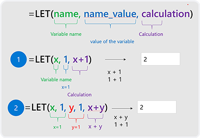
This function consists of 3 basic arguments. Name and value arguments can be optionally increased.
The 3 basic arguments are required. For the function to work, there has to be indicated value and calculation arguments.
Let’s take a look at these arguments.
- name1: The name for the 1st value
- value1: The value to associate with the 1st name
- name2 (optional): Additional names
- value2 (optional): Additional values
- calculation: The calculation to perform. This is always the final argument and it can refer to any of the defined names in the LET.
Deconstructing the parameters, there are two things to make note of
- The names and their values must be in pairs. If there is a name but there is not a value, the function doesn’t work.
- The last parameter of the function is the calculation which can use the values you named. A properly structured LET will have an odd number of arguments.
ADDITIONAL REMARKS
- The last argument should be a calculation that returns a result.
- Argument names are limited with the names that can be used in the Name Manager. For example, “a” is valid but “c” will not be a valid name since it coincides with the R1C1 reference styles.
This example will help you comprehend it better:
=LET(total; SUM(A1:A10); total * 3)
Let me give another example so that the software people can comprehend it better: in the formula below, I have created a variable called sum and gave it the 1 value. In the calculation part, I said add +2 to the sum variable and as a result, this function will return the result of 3.
=LET(SUM; 1; SUM+2)
If we want to take this a step further, I mean if we want to give double names and values, we can use it like this:
=LET(total, SUM(A1:A10), count, COUNT(A1:A10), total / count)
Here is another example:
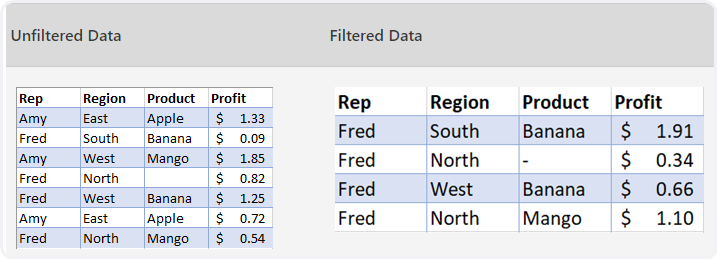
Here, you need to FILTER the Fred in the first column with the new FILTER dynamic string and if there is a blank cell, you need to enter – (hyphen) icon.
Normally, we can solve this with a formula like this; if there is a blank cell in the result coming from the filter, write hyphen there, if there is no blank cells filter normally.
=IF(ISBLANK(FILTER(A2:D8;A2:A8="Fred"));"-";FILTER(A2:D8;A2:A8="Fred"))
But if you have noticed, we wrote this part twice in the formula; FILTER(A2:D8;A2:A8=”Fred”)
LET function says that you don’t need to write the same data twice.
=LET(filterCriteria, “Fred”, filteredRange, FILTER(A2:D8,A2:A8=filterCriteria),
IF(ISBLANK(filteredRange),”-“,filteredRange))
Let me give another example of this beautiful function and than end my article: 😊
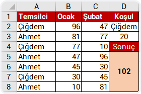
The formula we need to write when we want to find the total data of February based on the conditions indicated above in D2 and D3 in the table above:
=IF(SUMIFS($C$2:$C$8;$A$2:$A$8;$D$2;$B$2:$B$8;">="&$D$3)<0;"Sum Incorrect";SUMIFS($C$2:$C$8;$A$2:$A$8;$D$2;$B$2:$B$8;">="&$D$3))
As you can see, we used SUMIFS two times in IF. We had to write it like that depending on our need.
But if we are to do it with the LET function, we only need to write the SUMIFS function once.
=LET(Sum;SUMIFS($C$2:$C$8;$A$2:$A$8;$D$2;$B$2:$B$8;">="&$D$3);IF(Sum<0;"Incorrect";Sum))
So much for the information I will share with you for now. If you want you can get more information here. As we start using this function in our daily lives, we will be sharing it with you. ⚡️
See you in other articles, bye. 🙋🏻♂️
You can share this post with your friends and help them get informed as well.👍🏻