The RANDARRAY Function

In this article, I will be talking about one of the new dynamic array functions: the RANDARRAY function. Sometimes we need a data table filled out with random data. With this function, you can quickly fill as many rows and columns with numeral data. And you can find our articles about other functions on our blog.

WHAT DOES IT DO

The RANDARRAY function returns an array of random numbers. You can specify the number of rows and columns to fill, minimum and maximum values, and whether to return whole numbers or decimal values. The function returns a random set of values between 0 and 1 if you don’t enter an argument. For example, you can create a 20-row and 5-column table that contains whole numbers between 50 and 500 quickly in a few seconds.You will see an example below.

SYNTAX

=RANDARRAY([rows],[columns],[min],[max],[whole_number])This function has 5 arguments.
All of them are optional.

Now, let’s take a look at these arguments and what they mean, and what we will give them.

[rows]

Optional

The number of rows to be returned
[columns]

Optional

The number of columns to be returned
[min]

Optional

The minimum number you would like returned
[max]

Optional

The maximum number you would like returned
[whole_number]

Optional

Return a whole number or a decimal value

  • TRUE for a whole number
  • FALSE for a decimal number.


WORKING CONDITIONS

  • If you don’t input a row or column argument, RANDARRAY will return a single value between 0 and 1.

  • If you don’t input a minimum or maximum value argument, RANDARRAY will default to 0 and 1 respectively.
  • The minimum number argument must be less than the maximum number, otherwise RANDARRAY will return a #VALUE! error.

  • If you don’t input a whole_number argument, RANDARRY will default to FALSE, or decimal value.
  • The RANDARRAY function will return an array, which will spill if it’s the final result of a formula. This means that Excel will dynamically create the appropriate sized array range when you press ENTER. If your supporting data is in an Excel table, then the array will automatically resize as you add or remove data from your array range if you’re using structured references. For more details, see this article on spilled array behavior.

  • RANDARRAY is different from the RANDfunction in that RAND does not return an array, so RAND would need to be copied to the entire range.
  • An array can be thought of as a row of values, a column of values, or a combination of rows and columns of values. In the example above, the array for our RANDARRAY formula is range D2:F6,or 5 rows by 3 columns.
  • Excel has limited support for dynamic arrays between workbooks, and this scenario is only supported when both workbooks are open. If you close the source workbook, any linked dynamic array formulas will return a #REF! error when they are refreshed.


USE OF THE FUNCTION

Now, let’s see how this function works with 3 different examples. First, we will determine rows and columns. And then we will give row, column, min and max number values and return a retrospective array. And then, we will request the numbers to be returned to be whole number. The image we will obtain is going be like this:


excel rasgdizi farklı örnekler


See you in other articles, bye. 🙋🏻‍♂️
You can share this post with your friends and get them informed as well. 👍🏻


Office Insider – What Happened in March?

NEW FEATURES/FIXES


You can find and follow all monthly Office insider new features and fixes (updates) on our blog. 👍🏻  Officer insider gets updates and new features regularly. It is important to follow these Office insider updates and use them in terms of increasing your knowledge. Now let’s take a look at what kind of changes happened in Office insider in the month of March.


March 28, 2020

outlook iconOutlook

Calendar visual refresh

Last year, we brought you a refreshed mail experience, and, this year, it is the calendar’s turn to get a facelift! The updates are fresh but familiar so, as a seasoned Outlook user, you can jump in and be more productive right away.

Learn more.

Takvimde çalışma haftasının resmi.

Notable Fixes

  • This change addresses delays when processing images with malformed or invalid protocol information.
  • This change fixes an issue where the latest changes to draft emails were not being updated.
  • Fixed an issue where right-mouse clicking on a file and using ‘Send to’ would not work.
  • Fixed an issue where if a user had a customized the search path for the Address book, Outlook’s name resolution scope would be limited to the customized path rather than including the Global Address List (GAL).
  • Fixed an issue where within a set of returned search results, sorting the results by Categories would not display the Category colors.


PowerPoint iconPowerPoint

Synchronize changes while you are presenting

For years, PowerPoint didn’t allow changes made to slides by others to be displayed while presenting. This ensured that the presenter was in full control of the content being shared. No one could revise slides, either accidentally or maliciously. It also ensured that all of your computer resources were used for slideshow rendering. A concern that is especially important if you are running on a low-end machine.

However, while some presenters may still desire this original design, we’ve heard from others that they are seeking more flexibility. With an increased focus on collaboration and real-time updates, we’re excited to make available the ability to synchronize changes whenever they are made, even when the presentation is in Slide Show mode.


How it works

You can synchronize changes in two ways: automatically or manually.

Automatically update slide content

1. Select the Keep Slide Updated check box on the Slide Show tab on the ribbon.

PowerPoint

2. Start the presentation by selecting the appropriate button on the Slide Show tab.


Synchronize changes


3. Whenever an update to a slide is made and detected, the content is automatically updated and visible in the slide show being presented.

Manually update slide content

1. Clear the Keep Slide Updated check box on the Slide Show tab on the ribbon.

Synchronize changes


2. Start the presentation by selecting the appropriate button on the Slide Show tab.

3. Whenever an update to a slide is made and detected, an Update Slides button appears at the top of Presenter View.


Synchronize changes


4. Click the Update Slides button to manually synchronize the slide content.

word new iconWord

Notable Fixes

  • Fixed an issue where the functionality to post comments was disabled.
  • This change addresses delays when processing images with malformed or invalid protocol information.
  • This change addresses an issue where the account manager would not dispatch messages resulting in a hang with third party applications.
  • This change fixes an issue where the Table of Contents would get updated with heading styles which were not present in the document.
  • Fixed an issue where digital signatures saved in Word documents would be removed when mailing the documents.


excel new iconExcel

Notable Fixes

  • This change addresses delays when processing images with malformed or invalid protocol information.


msproject new iconProject

Notable fixes

  • Fixed an issue where the ‘ProjectBeforeTaskChange’ Visual Basic Applications (VBA) event did not fire when a user clicked the “Inactivate” button found on the Tasks Ribbon within the Scheduling grouping.
  • If you set predecessor or successor details from within a Form type view, the ProjectBeforeTaskChange Visual Basic Applications (VBA) event didn’t always capture the changes. For example, if you deleted a dependency and clicked OK on the form, the event did not fire. This behavior has been fixed.
  • Fixed an issue where the latest values for the Actual Cost of Work Performed (ACWP) would not be displayed after making a change, such as a date change.
  • Fixed an issue where opening a project using the Most Recently Used (MRU) menu opened the project file with Read/Write access.
  • This change fixes an issue where if you created a manual task with a start date and a time (but no duration), it would be displayed with an incorrect time on the timeline.
  • Fixed an issue where printing a timeline using Hijri calendar would result in a month being skipped or duplicated in the print view.
  • This change addresses an issue where working in Team Planner with GDI objects, could result in the over allocation of GDI objects and create low memory conditions.


March 13, 2020  

word new iconWord, excel new iconExcel,PowerPoint new iconPowerPoint andoutlook new iconOutlook

Sensitivity labels

You can now apply a sensitivity label that your organization has configured to prompt you for custom permissions. Learn more

How to Access

If your organization has set up Sensitivity tags in Microsoft Information Protection and enabled users to assign permissions, you can access them. For example, choose Home> Protect, then select the label you want to apply to the document, workbook, presentation, or email.

İzinlere nasıl erişileceğini gösteren Word belgesinin resmi.

outlook new iconOutlook

Notable Fixes

  • Addresses an issue that caused the “Last Modified”; date on a file to be updated when adding an attachment to a mail or saving an attachment from a mail by dragging and dropping it (as opposed to via a menu).
  • Addresses an issue that caused hitting enter in the expanded find pane to fail to start a search, requiring instead that users click on the search button.
  • Fixed an issue where search shows no information about users when the option to “Show user photographs when available” is disabled.


word new iconWord

Notable Fixes

  • Fixed an issue when typing or editing a comment and using Ctrl+A would result in selecting text in the canvas instead of selecting text just within the comment card.
  • We fixed an issue in which the alignment of words in a document gets scrambled when tried to edit after printing using Quick Print.
  • We fixed an issue when merging two documents into one document.
  • Fixed an issue where marking revisions involving equations could result in a failure when saving the file.


excel new iconExcel

Notable Fixes

  • Fixed a performance issue that users may have experienced when programmatically editing a large range of cells.
  • Fixed a performance issue that occurred when opening csv files with Japanese environments.


msproject new iconProject

Notable Fixes

  • Fixed an issue where summary task dates weren’t always getting calculated correctly.
  • Fixed an issue where the OnUndoOrRedo event doesn’t fire without first running the OpenUndoTransaction method.


access new iconAccess

Notable Fixes

  • Fixed an issue where international versions of Access were displaying English strings in the user interface.


PowerPoint

New Features

Look above.


March 10, 2020

excel new iconExcel,word new iconWord,PowerPoint andoutlook new iconOutlook

Pick the perfect color

We heard you! Converting Hex colors to RGB values is now a thing of the past. For any property where you can define a color, click the appropriate button in the ribbon (such as the Font Color button) and click More Colors. Then, in the Colors dialog box, click the Custom tab and enter the Hex color value in the Hex box, for example, #0F4C81 or 444.

Learn more

Onaltılık bilgiler alanını gösteren renkli kutu.

excel new iconExcel

Automatically use new data types*

When you type a data value that resembles a possible stock or geographic location, Excel offers to convert it to the appropriate connected data type – Stocks or Geography. Give it a try!

Type in several geographic locations (such as “Seattle”, “London”, or “Tel Aviv”) or stock ticker symbols (such as “MSFT”, “ADBE”, or “AAPL”) in separate cells in a column.

When Convert to Geography or Convert to Stocks appears to the right of the selected cell, click on it.

Verileri dönüştür kutusunun bulunduğu Excel çalışma kitabı.

* This feature is only available in English right now.

outlook new iconOutlook

Drag emails to a group you own

As a group owner, you can now move and copy messages and threads by dragging and dropping them from your mailbox to the groups’ mailbox. Once moved, the content is visible to all the group members, and anyone can read the messages and participate in the conversation.

Learn more

Better search results, faster

The Search experience in Outlook just got a facelift! It is now more reliable, intelligent, and faster than ever. Also, any search entry is now being spell checked and, if errors are detected, helpful suggestions are offered to ensure that you get to the results you’re looking for. Finally, notice that the most relevant search results are presented at the top of the results list, making access faster.

Arama öğelerinin vurgulandığı Outlook posta kutusu resmi.

PowerPoint

Diagrams get connector support

Now, the converted lines between objects are connectors anchored to the shapes.

Ink conversion is also easier than ever with just clicking the Convert your ink button Convert your ink button. Select the converted object again to be able to access other conversion alternates, to make sure the conversion fits your needs. Give it a try! Give it a try!

Sağda siyah bağlayıcı dönüştürme kutusuyla boş beyaz kutular.


March 6, 2020  

outlook new iconOutlook

Notable fixes 
  • We fixed an issue that was preventing users from attaching a file to their mail messages when that file was open in another application.
  • We fixed an issue where creating a rule with Outlook Web Access did not persist to the Exchange server and resulted in a conflict.
  • We fixed an issue with Outlook that wouldn’t show the drop-down list in the “From” field when using dark mode.


word new iconWord

Notable fixes 
  • We fixed an issue that made the User Principal Name (UPN) people case-sensitive, e.g., User.Name@microsoft.com would fail to match user.name@microsoft.com, and prevented users from accessing the SharePoint Sites service.
  • We fixed an issue that prevented the Compare feature from working when the document was protected for editing.


PowerPoint

Notable fixes 
  • We fixed an issue that made the User Principal Name (UPN) people case-sensitive, e.g., User.Name@microsoft.com would fail to match user.name@microsoft.com, and prevented users from accessing the SharePoint Sites service.
  • We fixed an issue where the recommended thumbnails flashed when hovering your mouse over the thumbnails. In some cases, this could cause PowerPoint to crash.


excel new iconExcel

Notable fixes 
  • We fixed an issue that made the User Principal Name (UPN) people case-sensitive, e.g., User.Name@microsoft.com would fail to match user.name@microsoft.com, and prevented users from accessing the SharePoint Sites service.


We compiled all the new features and fixes in March in Office insider. Hope to see you in our other articles, bye bye. 🙋🏻‍♂️
You can share this article with your friends and family to help them get information about Office insider updates released in the month of March. 👍🏻 

SELECT CASE DECISION STRUCTURE

In this article, I wanted to share some information about the Select Case Decision Structure which is one of the Decision (Condition) Structures in Excel & VBA, a.k.a Excel macros. You can find other articles about Excel & VBA on our blog.


WHAT IS THE SELECT CASE DECISION STRUCTURE?

The Select Case Decision Structure

can be used to control comparisons about a data, just like the IF structure.
The values it returns are going to be True or False. When it is True, the code lines under it work. When it is False, if there are other Case conditions, they are controlled.
If there are other Case conditions and they are True, the codes below them are applied.
If there is no other Case conditions or all the Case conditions have returned False, if there are other codes in the procedure, they are applied by getting out the block with End Select.

Even though it is similar to IF (IF Else ElseIf Then) its type is a bit different and if you have multiple conditions, it is way easier to use compared to IF.


Here is the Syntax..

Blue

parts cannot be changed.
Red parts can be changed.
Green parts are comment lines.

Select Case Data to be controlled
‘Your Codes
End Select

If we are going to have multiple conditions, than Case Is or Case statements come into the play. We also have the Case Else statement that allows us to say “do this if the controlled data is outside indicated conditions.”

Select Case Data to be controlled
Case Is Condition
‘Your codes
Case Is Condition
‘Your codes
Case Is Condition
‘Your codes
Case Else
‘Your codes
End Select

If you want, you can write to codes in the same row after the condition part with : (colon). Case Is Condition: Your Codes
If we use a comparison operator (<; <=; =; >; >=) while indicating a condition, Case Is statement is written for the condition. If not, Case statement will be enough. You will see this situation in the examples below.

We used this statement for the Select Case structure above: “If you have multiple conditions, it is way easier to use compared to IF.”
Let’s give an example of this. We will apply the same conditions with both the IF structure and the Select Case structure and see the difference.
Our conditions will be like this: we have a value and we’ll have it checked. If this value is smaller than 1, we will return the outcome with MsgBox. Likewise, if it is between 1 and 5 or 6 and 10 or 11 and 15, we’ll return the outcome with MsgBox. We will prepare this separately with both of the structures.


Let’s start. First, the codes that we will need if we write our codes depending on the conditions above with the IF structure are:

Sub IF_Yapisi_ile_1()
For i = 1 To 10
If Cells(i, 1).Value < 1 Then
MsgBox "Değer 1'den küçüktür."
ElseIf Cells(i, 1).Value >= 1 And Cells(i, 1).Value <= 5 Then
MsgBox "Değer 1 ile 5 arasındadır."
ElseIf Cells(i, 1).Value >= 6 And Cells(i, 1).Value <= 10 Then
MsgBox "Değer 6 ile 10 arasındadır."
ElseIf Cells(i, 1).Value >= 11 And Cells(i, 1).Value <= 15 Then
MsgBox "Değer 11 ile 15 arasındadır."
End If
Next i
End Sub


If we want to write our codes in different IF rows for each condition and simplify it, then we can write it like this:

Sub IF_Yapisi_ile_2()
For i = 1 To 10
If Cells(i, 1).Value < 1 Then MsgBox "Değer 1'den küçüktür."
If Cells(i, 1).Value >= 1 And Cells(i, 1).Value <= 5 Then MsgBox "Değer 1 ile 5 arasındadır."
If Cells(i, 1).Value >= 6 And Cells(i, 1).Value <= 10 Then MsgBox "Değer 6 ile 10 arasındadır."
If Cells(i, 1).Value >= 11 And Cells(i, 1).Value <= 15 Then MsgBox "Değer 11 ile 15 arasındadır."
Next i
End Sub


Now let’s see how we will write the same conditions with the Select Case statement.

Sub Select_Case_Yapisi_ile()
For i = 1 To 10
Select Case Cells(i, 1).Value
Case Is < 1: MsgBox "Değer 1'den küçüktür."
Case 1 To 5: MsgBox "Değer 1 ile 5 arasındadır."
Case 6 To 10: MsgBox "Değer 6 ile 10 arasındadır."
Case 11 To 15: MsgBox "Değer 11 ile 15 arasındadır."
Case Else: MsgBox "Değer 15'den daha büyüktür."
End Select
Next i
End Sub


We saw that we can execute the action we want with three different codes and we can increase this number, but I hope that you can see the difference between them.
With the IF structure, we had to indicate Cells(i, 1).Value –the cell address that we were going to have controlled and we wrote it many times to indicate the condition between two numbers. But with Select Case, it was enough for us to write the cell address that we were going to have controlled and it was very easy to indicate the condition between two numbers as 1 To 5.

Let’s see the outcome with the Select Case structure in a GIF.

select case karar yapısı vba


CODE SAMPLES

You can apply the Select Case application samples below and test how it works and comprehend its logic better.

Sub Makro1()
Select Case "Murat" = "Emre"
Case True: MsgBox "İfade Doğrudur."
Case False: MsgBox "İfade Yanlıştır."
End Select
End Sub


Sub Makro2()
Dim Değer As Integer
Değer = 2
Select Case Değer
Case 1: MsgBox "Değer 1'dir."
Case 2: MsgBox "Değer 2'dir."
Case 3: MsgBox "Değer 3'tür."
Case Else: MsgBox "Değer Mevcut Değil."
End Select
End Sub


Sub Makro3()
Dim Değer As Integer
Değer = 1
Select Case Değer
Case Is < 1: MsgBox "Değer Küçüktür."
Case Is = 1: MsgBox "Değer Eşittir."
Case Is > 1: MsgBox "Değer Büyüktür."
End Select
End Sub


Sub Makro4()
Dim Metin As String
Metin = "PEAKUP"
Select Case Metin
Case "Excel": MsgBox "Metin Excel'dir"
Case "PEAKUP": MsgBox "Metin PEAKUP'tır."
Case "VBA": MsgBox "Metin VBA'dır."
End Select
End Sub


Sub Makro5()
Dim Değer As Integer
Değer = 14
Select Case Değer
Case Is < 1: MsgBox "Değer 1'den küçüktür."
Case 1, 2, 3, 4, 5: MsgBox "Değer 1 ile 5 arasındadır."
Case 6, 7, 8, 9, 10: MsgBox "Değer 6 ile 10 arasındadır."
Case 11, 12, 13, 14, 15: MsgBox "Değer 11 ile 15 arasındadır."
Case Else: MsgBox "Değer 15'den daha büyüktür."
End Select
End Sub


Sub Makro6()
Dim Değer As Integer
Değer = 20
Select Case Değer
Case Is < 1: MsgBox "Değer 1'den küçüktür."
Case 1 To 9: MsgBox "Değer 1 ile 9 arasındadır."
Case 10 To 19: MsgBox "Değer 10 ile 19 arasındadır."
Case 20 To 29: MsgBox "Değer 20 ile 29 arasındadır."
Case Else: MsgBox "Değer 29'dan büyüktür."
End Select
End Sub


Sub Makro7()
Dim Değer As Long
Değer = 15
Select Case Değer
Case Is < 1: MsgBox "Değer 1'den küçüktür."
Case 1 To 4, 5 To 9: MsgBox "Değer 1 ile 9 arasındadır."
Case 10 To 14, 15 To 19: MsgBox "Değer 10 ile 19 arasındadır."
Case 20 To 24, 25 To 29: MsgBox "Değer 20 ile 29 arasındadır."
Case Else: MsgBox "Değer 29'dan büyüktür."
End Select
End Sub


Sub Makro8()
Dim Tanım As String
Tanım = "C"
Select Case Tanım
Case Is < "E": MsgBox Tanım & " harfi E harfinden önce gelir."
Case Is > "E": MsgBox Tanım & " harfi E harfinden sonra gelir."
End Select
End Sub


Sub Makro9()
Dim Tanım As String
Tanım = "E"
Select Case Tanım
Case "A" To "M": MsgBox Tanım & " harfi A ile M harfleri arasındadır."
Case "N" To "Z": MsgBox Tanım & " harfi N ile Z harfleri arasındadır"
Case Else: MsgBox "Case Else"
End Select
End Sub


You can cat more detailed information about the Select Case statement on Microsoft Docs.


See you in other articles, bye. 🙋🏻‍♂️
You can share this post with your friends and help them get informed as well.👍🏻

The SEQUENCE Function

In this article I will be talking about the SEQUENCE Function that is one of the dynamic array functions. It allows us to create a list of sequential numbers in an array when we want to give a sequence number in a column or we give a starting number and indicate the increase value. We can easily use it when we need to quickly create a data set. You can find articles about other functions on our blog.


WHAT DOES IT DO

The SEQUENCE Function -like I mentioned above- is a function similar to the Flash Fill option in the Fill field in Excel. For example, when we want to give a sequence number from 1 to 20, it is going to be enough for us to write =SEQUENCE(20). Or let’s say that you are going to create a 10-row and 5-column numeral data table. When we want these numbers to start from a certain number and increase by the value we indicate and fill the sequence like that, we can use this function. We can do extra special actions with the numeric values this functions returns us.


SYNTAX

=SEQUENCE(rows,[columns],[start],[step])

This function has 4 arguments.
The first one of these arguments is required and the other 3 are optional.

Now let’s take a look at what these arguments mean, i.e. what this function wants from us and what we will give it.

sıralı fonksiyon argümanları listesi


WORKING CONDITIONS

  • Any missing optional arguments will default to 1.
  • An array can be thought of as a row of values, a column of values, or a combination of rows and columns of values. In the example above, the array for our SEQUENCE formula is range C1:G4.

  • The SEQUENCE function will return an array, which will spill if it’s the final result of a formula. This means that Excel will dynamically create the appropriate sized array range when you press ENTER. If your supporting data is in an Excel table, then the array will automatically resize as you add or remove data from your array range if you’re using structured references. For more details, see this article on spilled array behavior.
  • Excel has limited support for dynamic arrays between workbooks, and this scenario is only supported when both workbooks are open. If you close the source workbook, any linked dynamic array formulas will return a #REF! error when they are refreshed.


USE OF THE FUNCTION

If you want, you can try to give a sequence number in a column. We can obtain a sequence of numbers starting from 1 for the specified number of rows and columns. If you wish, you can increase step by step by using the increment value. Let’s take a look at how to use the function.

sıralı fonksiyonu kullanımı


SPLIT THE DATA INTO COLUMNS EASILY

Now let’s have an example of the use in extra special actions…
Let’s assume that there are dozens, hundreds, thousands of row of data in the A column, and you want to split that data into a few columns. Now, we can create the list easily with the numbers it returns with the logic of this function. In the example below, there are 16 rows of data in the A column. Let’s get these written equally in the A and B columns with a row gap.


sıralı function farklı kullanımı


See you in other articles, bye. 🙋🏻‍♂️
You can share this article with your friends and help them get informed. 👍🏻

coder by

MASS E-MAIL WITH EXCEL THROUGH OUTLOOK

In this article, I will be talking about how we can execute an action which I know that many users need in Excel Training. Without further ado, let’s see how we can send a mass e-mail with Excel through Outlook.

excel toplu mail

First of all, we will be sending mass e-mails with Excel through Outlook with the power of VBA, a.k.a macros. So, it wouldn’t hurt you to know a bit about macros but I will be explaining the topic simply and since a lot of the code lines are cliche, it is not a must for you to know about macros. Also, I will be indicating what each code line means. First, I will give you all the codes. And then I will be explaining them. Of course, it can be enhanced way more but for now I will be explaining how to send a mass e-mail with a simple method. In addition, I will attach a sample file.

Let’s start.👍🏻


First, let’s assume that we have a table like this.
When we push the Send button, we will send all the e-mails starting from the 2nd row to the last row.

excelvba mail listesi


Send a Mass E-Mail with Excel through OUTLOOK – ALL CODES

Sub PEAKUP_Mail_Send()
   Dim Outlook As Object, newAs Object, i As Long
   Set Outlook = CreateObject("Outlook.Application")
   For i = 2 To Cells(Rows.Count, "A").End(3).Row
      Set new = Outlook.CreateItem(0)
      With new
         .To = Range("B" & i).Value
         .Subject = Range("C" & i).Value
         .Body = Range("D" & i).Value
         .Display
         '.Send
     End With
   Next i
   Set Outlook = Nothing: Set new= Nothing: i = Empty
   MsgBox "Your e-mails have been sent.", vbInformation, Application.UserName
End Sub

Yeap, these codes are all we need. Now, let’s move on to what each code line does. As I stated below, you can think of all the codes below as a template/cliche. It will be enough for you to take these codes and set to, subject and description parts according to your file.


Sub PEAKUP_Mail_Send()

We name our Macro/Procedure PEAKUP_Mail_Send.

Dim Outlook As Object, new As Object, i As Lon

We define the variables we’ll use. It is not a must to define variables but it is pretty helpful. I will be talking about the details in our article about variables and defining methods.

Set Outlook = CreateObject("Outlook.Application")

We created the Outlook application with the Late Binding method. (There are two methods; Early Binding and Late Binding)

For i = 2 To Cells(Rows.Count, "A").End(3).Row

We create a For loop from the 2nd row to the last filled row number in the A column. We use it to send the mail to all the addresses in all rows.

Set new= Outlook.CreateItem(0)

We create a new mail by setting just like pushing the New button in Outlook.

With new

Since the codes below indicate the fields in the new mail, in order not to write “new” each time, we say With new and indicate that it has to do with the new mail. If you pay attention, the codes continue as .To  – .Subject. So, they are all lines about the New mail.

.To = Range("B" & i).Value

We determine who we’ll send the mail to. Here we indicate that it will be sent to those on the B column.

.Subject = Range("C" & i).Value

We determine the subject. We indicate that the subjects are the ones on the C column.

.Body = Range("D" & i).Value

And we request the ones on the D column to be written into the mail body.

.Display

It enables you to display the mail before you send it.

.Send

Sends the mail.

End With

We must close the With statement with End With.

Next i

We request it to move on to the next line in the loop.

Set Outlook = Nothing: Set new= Nothing: i = Empty

We empty the created variable. It is not a must, but helps to not hold up space in storage.

MsgBox "Your e-mails have been sent.", vbInformation, Application.UserName

With MsgBox, we get a information window indicating that mails have been sent.

End Sub

We end our macro/procedure.


ADD EXTRA INFORMATION TO THE MAIL

Add a File

If you want, you can add a file in your computer with the code below to your mail. You can write the code line below under the .To – .Subject statements.

.Attachments.Add "file location"

Make the Look of The Text in the Message Body HTML

Instead of using .Body and writing a plain text, you can use .HtmlBody and make the text visually pleasing with html tags.

For example;

.HTMLBody = "

Add CC and BCCIf you want to add other people to the CC or BCC, you can write these codes under the .To line..CC = “Mail address to be added to CC .BCC = “Mail address to be added to BCCSet the Importance of the MailIf you want to send your mail with high importance, you can add this code line..Importance = 2
Well… if you have analyzed and learned everything I have written so far, we can move on to the application part. 😃
When we run the codes, the mails will be sent to all the addresses like in the GIF below.Note: If you activate .Send instead of .Display, the mails will be sent without displaying. excelvba outlook ile mail göndermek
You can download the application file here 👉🏻  .
And here is another example for you.
See you in other articles, bye. 🙋🏻‍♂️
You can share this post with your friends and help them get informed as well.👍🏻

Hello,
” & Range(“D” & i).Value & “

CREATE CUSTOM LISTS IN EXCEL

In this article, we will be talking about how to create a Custom Menu depending on your needs in Excel without any codes. You can find articles about other features on our blog.


ENJOY YOUR OWN CUSTOM LIST

As you know, there are a lot of menus and tons of features in those menus in Excel, from File Menu to Help menu. Sometimes we spend a lot of time looking for a feature in menus or there are features in menus that we don’t use at all. And sometimes, we are just up for a change. 😃 In all these case, you can create your own custom menu and place it anywhere you want, and just do all actions within that menus. And on top of that, you don’y need any UI Editor to execute this action.

özel menü


WHERE TO START?

To create a custom menu, we need to go to the  Customize Ribbon field in the Excel Options. There are two ways to go there.

The 1st way:

  • File
  • Options
  • Customize Ribbon


The 2nd way: 

  • Customize Quick Access Toolbar
  • Other Commands
  • Customize Ribbon


The window we’ll access through both ways will be this one.

şeridi özellştir


Come to this window, choose the Help menu and create a new tab/menu by clicking the New Tab button.

Choose New Tab (Custom), click “Rename” and name the new tab. For example, let’s type in PEAKUP. You can choose “New Group” and name it based on the features you’ll add. For now, we can call it Data Analysis.

Now we can add the features/commands we use the most to this menu.


If you want, you can do all the actions we’ve covered so far like in the image below.

özel menü ekle


If you right-click the Data Analysis group and choose Hide Command Labels options,


komut etiketlerini gizle

Your command will be seen as mini commands in the menu like this.mini etiket


You can add multiple groups into a menu by creating New Groups. Or you can create New Menus with the New Tab button and place it in the first place after the File menu.

özel menü yeni

I say create menus like this for a while and just try it out. 😄 You can check here for more details.


See you in other articles, bye. 🙋🏻‍♂️
You can share this post with your friends and help them get informed as well.👍🏻

LET : THE NEWEST FUNCTION

This week I will be talking about a function recently announced by Microsoft that only the Office Insider users can use: the LET Function. Like I mentioned in the FILTER function article, as the new dynamic string functions we will be able to execute a lot of actions more simply and quickly. And new features keep coming one after another. You can easily keep up-to-date by following our articles. 👍🏻


DEFINITION OF THE LET FUNCTION

In the announcement the definition goes like:

Have you ever had to repeat the same expression multiple times within a formula, created a mega formula or wished that you had a way to reuse portions of your formula for easier consumption? With the addition of the LET function, now you can!

The LET function assigns names to calculation results and makes it easier for you to reuse the parts of the formula. In a way, it means that we can Define Names in a function and use the name in calculation. Sometime when we are writing a formula, we need to state the same range or condition multiple time. the LET function will be helping as right at this point. We will name the value we have to use multiple times in a formula and we’ll indicate it with that name in the function.

The main benefits are:

1. Readability

No more having to remember what a specific range/cell reference referred to, what your calculation was doing or duplicating the same expression within a formula. With the ability to name expressions, you can give meaningful context to readers of your formula.

2. Performance

If you reuse the same expression multiple times in a formula, Excel calculates that expression multiple times. LET allows you to name the expression and refer to it using that name. Any named expression is calculated only once, even if it is referred to many times in the formula. This can significantly improve performance for computationally complex expressions.


SYNTAX

LET

(name1, value1, [name2…], [value2…], calculation)

let fonksiyonu

This function consists of 3 basic arguments. Name and value arguments can be optionally increased.

The 3 basic arguments are required. For the function to work, there has to be indicated value and calculation arguments.

Let’s take a look at these arguments.

  • name1: The name for the 1st value
  • value1: The value to associate with the 1st name
  • name2 (optional): Additional names
  • value2 (optional): Additional values
  • calculation: The calculation to perform. This is always the final argument and it can refer to any of the defined names in the LET.


Deconstructing the parameters, there are two things to make note of

  1.  The names and their values must be in pairs. If there is a name but there is not a value, the function doesn’t work.
  2. The last parameter of the function is the calculation which can use the values you named. A properly structured LET will have an odd number of arguments.


ADDITIONAL REMARKS 

  • The last argument should be a calculation that returns a result.
  • Argument names are limited with the names that can be used in the Name Manager. For example, “a” is valid but “c” will not be a valid name since it coincides with the R1C1 reference styles.


This example will help you comprehend it better:

=LET(total; SUM(A1:A10); total * 3)

Let me give another example so that the software people can comprehend it better: in the formula below, I have created a variable called sum and gave it the 1 value. In the calculation part, I said add +2 to the sum variable and as a result, this function will return the result of 3.

=LET(SUM; 1; SUM+2)

If we want to take this a step further, I mean if we want to give double names and values, we can use it like this:

=LET(total, SUM(A1:A10), count, COUNT(A1:A10), total / count)

Here is another example:

izinver fonksiyon örneği

Here, you need to FILTER the Fred in the first column with the new FILTER dynamic string and if there is a blank cell, you need to enter – (hyphen) icon.

Normally, we can solve this with a formula like this; if there is a blank cell in the result coming from the filter, write hyphen there, if there is no blank cells filter normally.

=IF(ISBLANK(FILTER(A2:D8;A2:A8="Fred"));"-";FILTER(A2:D8;A2:A8="Fred"))

But if you have noticed, we wrote this part twice in the formula; FILTER(A2:D8;A2:A8=”Fred”)

LET function says that you don’t need to write the same data twice.

=LET(filterCriteria, “Fred”, filteredRange, FILTER(A2:D8,A2:A8=filterCriteria),

IF(ISBLANK(filteredRange),”-“,filteredRange))


Let me give another example of this beautiful function and than end my article: 😊

izinver fonksiyonu

The formula we need to write when we want to find the total data of February based on the conditions indicated above in D2 and D3 in the table above:

=IF(SUMIFS($C$2:$C$8;$A$2:$A$8;$D$2;$B$2:$B$8;">="&$D$3)<0;"Sum Incorrect";SUMIFS($C$2:$C$8;$A$2:$A$8;$D$2;$B$2:$B$8;">="&$D$3))

As you can see, we used SUMIFS two times in IF. We had to write it like that depending on our need.

But if we are to do it with the LET function, we only need to write the SUMIFS function once.

=LET(Sum;SUMIFS($C$2:$C$8;$A$2:$A$8;$D$2;$B$2:$B$8;">="&$D$3);IF(Sum<0;"Incorrect";Sum))


So much for the information I will share with you for now. If you want you can get more information here. As we start using this function in our daily lives, we will be sharing it with you. ⚡️


See you in other articles, bye. 🙋🏻‍♂️

You can share this post with your friends and help them get informed as well.👍🏻

The Weekday Function

In this article, I will be talking about on of the Date and Hour functions, the WEEKDAY Function that will helps us in our daily lives. This function returns the number that represents the day of the week of a specific date. It gives us a number between 1 and 7, and so we know which day of the week it is and do actions depending on that. If you want, you can get the details about the Weekday Function on support office. You can find our articles about the other function on our blog


WHAT DOES THE WEEKDAY FUNCTION DO?

The WEEKDAY Function

gives us a number stating the which day a date is in that week. For example, If we want to know which dates in a column are weekend, we can have them highlighted. Or, doesn’t matter which day the payment days are in the column, if your payment day is Friday you can organize all the dates on Friday in their weeks.

SYNTAX

WEEKDAY(serial_number,[return_type])

The WEEKDAY Function

has 2 arguments.
The first one of them is required and the other one is optional.

Now let’s take a look at the meaning of these arguments, i.e. what this function wants from us and what we will give it.

haftanıngünü fonksiyonu argüman listesi


WORKING CONDITIONS

The working conditions of the WEEKDAY function are:

  • Microsoft Excel stores dates as sequential serial numbers so they can be used in calculations. By default, January 1, 1900 is serial number 1, and January 1, 2008 is serial number 39448 because it is 39,448 days after January 1, 1900.
  • If serial_number is out of range for the current date base value, a #NUM! error is returned.

  • If return_type is out of the range specified in the table above, a #NUM! error is returned.

  • If the Calendar is Gregorian, the returned number represents the Gregorian day of the week.
    If the calendar is Hegira, the returned number represents the Hegira day of the week. If the calendar is Hegira Calendar,  the argument number is any number that can represent a date and/or time from 1/1/100 (Gregorian Aug 2, 718) to 4/3/9666 (Gregorian Dec 31, 9999).


USING THE WEEKDAY FUNCTION

In the Weekday Function, we choose the date that we want to get the day number for the Serial_number argument first. Then, we choose the type that we want the Return_type argument to return. We will come across the list where the first and last days of the week are stated. For us the option is the one with the number 2, where first day is Monday and the 7th day is Sunday. So, we choose the 2 option for the return_type argument and complete the formula.


 HIGHLIGHTING THE WEEKENDS

Let’s assume a list in which there are dates of March in a column. At the first glance, we cannot know which day those dates are. If you choose that column, choose Long Date as Format in the Number group in Home menu, you will get the day name and it might be useful for you. But we don’t want the day name, we want the weekends to be highlighted. We can achieve this with the WEEKDAY Function in the Conditional Formatting feature. Colors are very useful when it comes to analyzing a data.

Let’s start practicing with examples. You can apply these steps with me.
Unfortunately, an available rule that does what we want doesn’t exist in Conditional Formatting.
So, what do we do? We create our own rules with a formula, and achieve highlights based on that rule.
You can find and highlight the weekends like this.

weekday fonksiyon kullanımı


SETTING THE PAYMENT DAY AS FRIDAY

Let’s do an example of setting the payment day as Friday.
For this action, we will use the CHOOSE and WEEKDAY functions together.
Try to do this action as well and try to comprehend its logic by repeating few times.

weekday ile ödeme gününü cuma gününe ayarlama


See you in other articles, bye. 🙋🏻‍♂️
You can share this post with your friends and get them informed as well. 👍🏻

Methods of Declaring VBA Variables

In this article, we will be talking about Declaring VBA Variables. Variables are essential elements of programming. Using and managing variables are one of the musts while creating a project. I will try my best to tell it as simple as possible. Reminder: You can find other articles about VBA on our blog. 👍🏻


About Declaring VBA Variables

Variables are usually used to store a data and use it when necessary. They are usually separated into two classes. Global variables and Local variables. Global variables can be used by all the functions of the program, but the local variables are used by the functions that have declared them.

It can be called back, reassigned or fixed during the execution of a procedure, function or module.
Declaring a variable will enable you to indicate the names of the variable you’ll use and the data type the variable will contain.

For example, if Result = 10, the variable Result can be declared as Integer Whole Number .

We usually name the variables in a short and easily remembered way. The most frequently used variable names are one character names like i, a, n, x ,y ,z, s so that it is easy to write in the code. If the variable name is a name that you can remember while using in the code, the probability of making a mistake while writing the code decreases.

Now we can move on to the declaring part.


The syntax concerning declaring variables is usually like this.
Dim variable_name [(stringsize)] As type
Public variable_name[(stringsize)] As type
Static variable_name[(stringsize)] As type


Along side this general declaring, the declaring methods below can be used as well.

  1. Declaring with Dim
  2. Declaring with Data Indicators (Abbreviations)
  3. Declaring with DEF

Declaring with Dim

It is the most known and used VBA Variable Declaring method.

We indicated the syntax Syntax below. Let’s make it clear with a few examples. Let’s say that we will declare a variable named row to use in the rows (cells) in the A column. Since the row numbers are whole numbers, we can used one of the whole number types we’ve indicated in our Data Types article. It would be better to use the variable data type depending on the row number we’ll get controlled or the maximum number that can be in the cell.

As well as we can use as Number or Whole Number, we have 3 basic variable data types: ByteInteger and Long. If the number we’ll assign to the row variable is 255 or less, then we can use the Byte variable data type. If the number we’ll assign to the row variable is between –32767 and+32768, then we can use the Integer variable data type. If it can be a bigger whole number, then we should use the Long variable data type. If a bigger number than what the variable can contain is sent, that the Overflow error occurs. And if a text data is sent to a variable that was determined as number, Type Mismatch error occurs.


Let’s give a few examples of declaring variables with Dim:

Sub PEAKUP()
    Dim row As Long
    Dim column As Byte
    Dim text As String
    Dim start As Date
    Dim money As Currency
    Dim object As Object
    row = 15
    column = 5
    text = "Excel Turkey Forum"
    start = "24.06.2018"
    money = 300
    Set object= ActiveSheet
End Sub

We can write each variable one by one in different rows like that, but we also can write them side by side like this. We just need to put Dim in the beginning and put a comma between each variable.

Sub PEAKUP()
    Dim row As Long, column As Byte, text As String
    Dim start As Date, money As Currency, object As Object
End Sub

We need to be careful about this here: Some users make a mistake and declare incorrectly.

If you write the code I gave above like this one below, I mean if you start with Dim and think that you’ve declared the first variable and not declare the other variables with the suitable variable data types. Since in the “column”, “text” variable the data type is not stated, Byte and String are not indicated but Variant is -which is undefined data type. Since in the first variable I’ve declared with Dim, you declare the data type in the first variable. So, it doesn’t mean that you declare the next variables as well. You need to state the data type of each variable one by one.


Declaring with Data Identifiers (Abbreviations)

Abbreviations 

They are also known as Type Indication suffixes.
They are not used much but they help to save in codes.
It is also possible to tell a variable type by adding a special character to the end of the variable name in VBA.

Dim number% 'Integer
Dim longnumber& 'Long
Dim sum! 'Single
Dim subtotal# 'Double
Dim payment@ 'Currency
Dim name$ 'String
Dim longestnumber^ ' 64 bit LongLong


Data Type Abbreviation Characters

VBA

, as a fast way of declaring data type, lets you add a character in the name of a variable.
This method shouldn’t be used to declare variables and it can be used for retrospective purposes only.
The row below will declare a Double data type and a variable.

Dim dDouble#

But it is better for this row to be declared with the “As” keyword.
Dim dDouble As Double


Data Type Abbreviation/ Suffixes

If you you abbreviations, you don’t have to declare the type.
If you use the % expression, you don’t need to write “As Integer”.
These abbreviations can be helpful to get available information to Variants.

For example: count =10#


Declaring with DEF

We can declare our variables with different methods like we mentioned, one of these methods is declaring with DEF.
This declaration is usually done free from the procedure at the top of the code window.
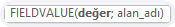
We can abbreviate and declare the data type we use as variable like below.
The letter that comes after Def+Type indicated that the variables starting with that letter belong to that type.

def ile değişken tanımlama tablosu

Let’s see an example that shows the difference between declaring with Def and Dim.

First, let’s declare our variables like this with Dim.

Sub PEAKUP()
    Dim row As Integer, column As Integer
    Dim text As String, letter As String, word As String
    Dim date As Date, start As Date
    Dim number As Double, price As Double
    row= 10
    column= 5
    text = "PEAKUP"
    letter = "E"
    word = "Book"
    date = "24.06.2018"
    start = "14.12.1980"
    number = 1453.48
    price = 5647.15
End Sub

Now, let’s do the same declaration with Def.

DefInt R
DefStr L, W, T
DefDate S, D
DefDbl P, N
Sub PEAKUP()
    row = 10
    column = 5
    text = "PEAKUP"
    letter = "E"
    word = "Book"
    date = "24.06.2018"
    start = "14.12.1980"
    number = 1453.48
    price = 5647.15
End Sub

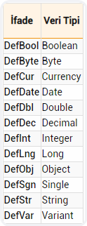
As you see, we got to indicate the type by using the initials and declare the variables. At this point, you want the variable declarations not to take too much space and be seen in less rows. As indicated below, you can write the Def rows in a row next to one other with a colon (:).

DefInt R: DefStr L, W, T: DefDate S, D: DefDbl P, N
Sub PEAKUP()
    row = 10
    column = 5
    text = "PEAKUP"
    letter = "E"
    word = "Book"
    date = "24.06.2018"
    start = "14.12.1980"
    number = 1453.48
    price = 5647.15
End Sub

By the way, you can easily follow and evaluate the names, values and types of all variables from Locals Window.

def ile değişken tanılamayı locals windowda görüntüleme


You can take a look at the Microsoft Docs page for more information.

See you in other articles, bye.🙋🏻‍♂️
You can share this post with your friends and get them informed as well. 👍🏻

FIELDVALUE Function

In this article, we will be informing you about the FIELDVALUE Function used with the Linked Data Types. You can use the FIELDVALUE function to retrieve field data from linked data types like the Stocks or Geography data types.

bağlantılı veri türleri

There are easier methods for writing formulas that reference data types, so the FIELDVALUE function should be used mainly for creating conditional calculations based on linked data types.


SYNTAX

fieldvalue fonksiyonu söz dizimi

This function requires two arguments.
It is necessary to enter both of these arguments.

There are these independent variables in the syntax of the FIELDVALUE function:

  • value– Function returns all matching fields(s) from the linked data type specified in the value argument.
  • field_name– The name or names of the fields you would like to extract from the linked data type.

Description

  • The FIELDVALUE function returns all matching fields(s) from the linked data type specified in the value argument.

  • The FIELDVALUE function belongs to the Lookup & Reference family of functions.


Examples

In the following basic example, the formula =FIELDVALUE(A2,”Area”) extracts the Area field from the geography data type for Turkey.

fieldvalue fonksiyonu örnek

Let’s list the data in the related field depending on the dynamic field choice about cities.

fieldvalue fonksiyonu örnek


Remarks

If you try to retrieve data from a non-existent data type field, the FIELDVALUE function will return the #FIELD! error. For instance, you might have entered “Field“, when the actual data type field is named “Area“. Double-check your formula to make sure you’re using a valid field name. If you want to display a list of field names for a record, select the cell for the record, and press Ctrl+Shift+F2 .

You can get more information on Microsoft Support.

See you in other articles, bye. 🙋🏻‍♂️
You can share this post with your friends and help them get informed as well.👍🏻