Tag: file trickster

EXCEL’S HISTORY (EXCEL FROM PAST TO TODAY)

EXCEL’S HISTORY (Excel from Past to Today)

Hello everyone,

I received a lot of questions like “Who found Excel, how was it created? It develops all the time, I wonder how the first version was…” in many of the trainings I gave in corporate companies.

As an answer to there questions, I have prepared the history of Excel and wanted to take the old users to a time travel that would make them say: “”Oh! What times…” And it will serve as an informative article for the new users.

Are you ready for the time travel? 👨🏻‍🚀

We met the first Excel as VisiCalc in 1978.
In 1978, Harvard Business School students Dan Bricklin ^{Father of the modern Excel}had to take on an analysis task for a case study. He had two alternatives to do that:

He would do it manually.
He would use a simple and unskillful computer program.

He thought that he didn’t have a better alternative and chose VisiCalc in the 1978 fall.
He programmed the first study and prepared the prototype of the concept he called VisiCalc. The first version of VisiCalc was a matrix of 4 columns and 20 rows.
It was not close to the electronic tables of our day but VisiCalc was still an accomplishment for that moment.

That was the first electronic table program and was published for Apple II at first.
It had skills like basic arithmetic operations, recalculating instantly and scroll bars.

1978 – VISICALC

1980 – SUPERCALC

1982 – MULTIPLAN

1983 – LOTUS 1-2-3

1985 – MICROSOFT EXCEL 1.0 (MAC)

1987 – MICROSOFT EXCEL 2.0 (WINDOWS)

1990 – MICROSOFT EXCEL 3.0

1992 – MICROSOFT EXCEL 4.0

1993 – MICROSOFT EXCEL 5.0

1995 – MICROSOFT EXCEL 7.0 (Excel 95)

1997 – MICROSOFT EXCEL 8.0 (Excel 97)

1999 – MICROSOFT EXCEL 9.0 (Excel 2000)

2001 – MICROSOFT EXCEL 10.0

2003 – MICROSOFT EXCEL 11.0 (Excel 2003)

2007 – MICROSOFT EXCEL 12.0 (Excel 2007)

2010 – MICROSOFT EXCEL 14.0 (Excel 2010)

2013 – MICROSOFT EXCEL 15.0 (Excel 2013)

2016 – MICROSOFT EXCEL 16.0 (Excel 2016)

2019 – MICROSOFT EXCEL 16.0 (Excel 2019)

2019 – MICROSOFT EXCEL 16.0 (Office 365)

Now I leave you alone with the 1992 Microsoft Excel introduction..

Well, I hope that you enjoyed this few-minute trip to the past.
You can share this post and take a few more people to the past as well. 👍🏻

Good bye.

CREATE A SPEEDOMETER CHART

SPEEDOMETER CHART

Hello everyone,

In this article, we will create a Speedometer chart. We will see how to create it simply step by step. Let me tell you this first: Microsoft will add this Speedometer chart to the standard charts for Office 365 users. I will be talking about the simplest version until then. I have stated what to do step by step below, please try to practice those steps with me. After learning how to create this chart, you can take a look at our Mouse Over Dashboard article. 😉

Let’s get started. 👍🏻

Before we start creating the chart, we have to have suitable data. We can create this chart with a few methods. We will use a combo chart in a data table to execute this action the shortest way possible.

⚫️ Let’s have this data starting from A1.

Indicator	Index
25	0
35	2
40	100
100

⚫️ Choose any cell and click the Insert menu.

⚫️ Click Combo chart in the Charts group and then click Create Custom Combo Chart.

⚫️Choose the Chart Type of the Indicator as Doughnut on the Add Chart window that pops open. And choose the Chart Type of the Index as Pie and mark the Secondary Axis option, and then click OK.

⚫️ Click the + icon of the chart added to the page and unmark Chart Title and Legend.

⚫️ Right -click on the green area on the chart and then click Format Data Series. Make the Angle of the first slice 270 on the screen that opens up on right and press Enter.

⚫️ Go to Shape Fill in the Format menu and choose No Fill.

⚫️ Choose the Series “Indicator” option in the Current Selection field in the Format menu.

⚫️ Make the angle of the first slice 270 on the screen that pops open on right and then press Enter.

⚫️ We will remove the fill color of the purple piece at the bottom. For this press CTRL + ► (Right Key) 4 times and choose the purple Data Point and then go to Shape Fill in the Format menu and choose No Fill.

⚫️Now press CTRL + ► (Right Key) and choose the colors you want in the Shape Fill in the format menu for data points. If you want a bright image, you can use the Shape Effects. Note: If you click the same shape effect twice, it will become brighter.

⚫️ Choose the index only, right-click and add Data Labels. And then choose the data label and go to the formula bar, write equals to (=) and choose the B2 cell and press Enter. You can increase the font size of the data label and make it bold. The chart will look like this at this point.

⚫️If you want, you can add a Spin Button (Form Control) to the page that would make index move.

On the Developer tab, in the Controls group, click Insert, and then choose Form Controls and draw somewhere suitable in the page, for example to a blank area or a blank cell. Note: You can make the index bolder by increasing the number 2 that is indicated as the Index thickness in the cell B3.

⚫️ Right-click the form control item you’ve added and click Format Control. Go to Cell Link and choose the cell B2. And arrange the others values as the ones below.

⚫️Your Speedometer chart will be ready when you choose a circle among the Shapes and add into the middle of the chart.

Lastly, I want to share the file I have prepared with you.
You can download the file here. 👉🏻

You can share this article and help many other people get informed as well.

Goodbye. 🙋🏻‍♂️

chart Excel file trickster grafik hız göstergesi msexcel speedometer

THE TABLE FORMAT and ITS BENEFITS

In this article, we will be talking about the benefits of the table format of the data range in Excel. When we write titles and enter data under those title or when working on a prepared file we received, we say that we have prepared a table. But the data range we call a table is not a table for Excel yet. For it to be seen as a table, you need to format the data range as a table. At that point, it allows us to use a lot of features that table format allows us.

Now let’s take a look what we need to do before creating to table to use some features and how we do them after formatting as table. By the way, it would be very helpful to write the articles on our Blog when you have a chance. If you wish, you can read a detailed article on Office Support.

Choose Style for the Table Format

We can use this feature by choosing Format as Table in the Styles group in Home tab. Choose any cell on your data and click the Format as Table command and choose the table style you want. You will have turned your data into a table quickly. Don’t forget: Everything added to the page later is an object. An image, shape, chart, table, slicer etc. all of them are objects and a menu with features of objects added later is added to the Ribbon.

You can apply this feature easily with the shortcut keys.
Choose any cell on your data and turn your data into a table with the

CTRL + T

shortcut.

Now, let’s see what kind of features our data range gained with such a simple shortcut.

Benefits of the Table Format

When you choose a cell on the table and move upwards and downwards, the column titles will be the titles of your table. Thus, you don’t need to use the Freeze Top Row feature in the Freeze Panes field in the View tab.

A style is applied to our table automatically and each row is colored as dark and light successively one-by-one. And this creates a nice image.

When you keep entering data under the table or next to the table, your table gets longer and wider. And this enables the data we enter later to be included in the table and everything to be accepted as a whole.

Before applying the table format, when we want to get the 18% VAT in the Sum field written to the next column; we had to write the formula into a cell and drag it down first. If there are blank rows in between, we had do drag down again. But, when we format it as a table, it is enough to write the formula and press Enter for the formula to be applied on the whole column.

When we turn the data into a table, a menu named Table Design or just Design is created in the Ribbon. This menu contains the features that we can use for our table. One of the most important features is the Slicer feature that we are familiar with from the Pivot Table. This feature enables us to filter the area we want on our table with one click.

It allows us to add functions like sum, average, count, min, max easily when we filter on the table. You can take a look at the other Table Style Options.

When you create a Pivot Table from the data range, you have to choose Change Data Source most of the time when new data is added outside the field specified as the range. Considering that you add new data to your table every day, you will have to choose Change Data Source and specify the new data range all the time. But, when we turn our data into a table, the data we add under it or next to it will be accepted as a part of the table and is within the data range. Thus, it will be enough to Renew for the data to be reflected on the Pivot Table.

In the formulas, we get to specify the data range by writing the table’s name without having to choose the whole table.

We have seen a lot of positive features till now and we obtained them with CTRL + T only.

Big or small, we recommend you to use Format as Table while working with data.
This way, you will be able to use the features above that will make you gain visualization and speed.

Convert to Range

Lastly, when you want to convert your table to data range again, you have two options.

By choosing Convert to Range in the Table Design or Design menu.
By right-clicking a cell on the table and choosing Convert to Range from Table.

I hope that this was a helpful article for you.
You can share this article with your friends and help a lot of people get informed as well.

Good bye. 👍🏻

Excel file trickster msexcel office insider table table style tablo tablo biçim

CONCATENATE vs TEXTJOIN

Hello everybody!

In this article, I invite you to say goodbye to the old CONCATENATE function that when we wanted to add a space or any other character while concatenating the data, obliged us to do it one by one and thus that was very laboring, and say welcome to a more efficient function. If you need to join the data in multiple cells and add characters like a space, comma, semi colon, and hyphen; there is just one function that you need to use and that is the TEXTJOIN function.

WHAT DOES IT DO

Like I mentioned above, you don’t need to click cells one by one and use an expression like ;” “; to add a space in between each time or a statement like & ” ” & when joining with the & character in the textjoin function. It joins each cell in the selected cell range by adding the slicer we’ve indicated. This way, we can join the data in hundreds of cells easily as a text.

SYNTAX

TEXTJOIN(delimiter, ignore_empty, text1, [text2], …)

There are 3 main arguments in the function.

These 3 main arguments are required, the other arguments are optional.Now let’s take a look at what these arguments mean, i.e. what the function wants from us and what we will give it.

delimiter (required)	A text string, either empty, or one or more characters enclosed by double quotes, or a reference to a valid text string. If a number is supplied, it will be treated as text.
ignore_empty (required)	If TRUE, ignores empty cells.
text1 (required)	Text item to be joined. A text string, or array of strings, such as a range of cells.
[text2, …] (optional)	Additional text items to be joined. There can be a maximum of 252 text arguments for the text items, including text1. Each can be a text string, or array of strings, such as a range of cells.

WORKING CONDITIONS

If the resulting string exceeds 32767 characters (cell limit), TEXTJOIN returns the #VALUE! error.
It came with Microsoft Excel 2019. If you are using and older Office version, you will get the #NAME? error and thus not be able to use this function.
If you Office 2019 or Office 365, you can easily use this function.

USING THE FUNCTION

After we write the function name, we specify the delimeter. And then we will choose how it should behave about the possible blank cells in the cell range. And in the last arguments, we choose the cell range to be joined. Now, let’s take a look at its use together.

In the example below, we join the data between the A and G columns with a semi colon in between them.

As you see, it is as easy as that to join a multiple cell range in a single text with any character between them.

See you in another articles, bye. 🙋🏻‍♂️
You can share this post with your friends and help them get informed as well.👍🏻

Excel file trickster MetinBirleştir msexcel office insider Office365 textjoin

Office App Has Been Renewed for Android and iOS

New Office App

Hello everybody,

Working from home has been inevitable during these times where online working systems have become prominent and even an obligation. Being able to work on one application while a lot of digital applications come into our life makes us faster and most productive in business processes.

At this point, we can say that all applications have become more visually appealing since Microsoft started to use Material design. Of course they also added very successful features to all applications. Now; Excel, Word and PowerPoint seem to have come together in one Office App in both Android and iOS devices. Which means that you will be able to access you Excel, Word and PowerPoint apps in one application.

Excel, Word and PowerPoint in One Single App

View, edit and share documents without having to change between multiple apps. We recommend you to try this new experience with its design and new features. 👍🏻

You can download the new application here:

iOS: https://aka.ms/OfficeAppiOS
Android: https://aka.ms/OfficeAppAndroid

New Features

Create PDFs from images or Word, Excel and PowerPoint documents instantly.
Sign PDFs with your fingers.
Take quick notes with sticky notes.
Scan QR codes to open links.
Take a picture of a documents and turn it into an editable Word document with one button.
Turn a table’s picture to an Excel e-table to be able to work with your data.
Let PowerPoint help you to create a presentation by choosing the pictures you want to use from your phone.
Create advanced digital images of white boards and documents with the Office Lens features that are integrated to the app.

You will love the promotional videos.🤗

Excel file trickster msexcel msoffice Office office app Office365

IDEAS

In this article, I will be talking about the Ideas feature of Excel.

Explore your data in more detail with Ideas.

The Ideas button -one of the new features- explores the order within your data and offers smart and custom ideas by using that.
Ideas in Excel empowers you to understand your data through natural language queries that allow you to ask questions about your data.
Simply click a cell in a data range, and then click the Ideas button on the Home tab.
Ideas in Excel will analyze your data, and return interesting visuals about it in a task pane.

Creates dozens of artificial intelligence analysis and reports from the data in your table for you.

On which data do Ideas work?

Ideas work best when data is formatted as an Excel table with a single title row on top.

Here is an example:

Ideas works best with clean, tabular data.

Here are some tips for getting the most out of Ideas:

Ideas works best with data that’s formatted as an Excel Table. To create an Excel Table, click anywhere in your data and then press Ctrl+T.
Make sure you have good headers for the columns. Headers should be a single row of unique, non-blank labels for each column. Avoid double rows of headers, merged cells, etc.
If you have complicated, or nested data, you can use Power Query to convert tables with cross-tabs, or multiple rows of headers.

Didn’t get Ideas?

Here are some reasons why Ideas may not work on your data:

Ideas doesn’t currently support analyzing datasets over 1.5 million cells. There is currently no workaround for this. In the meantime, you can filter your data, then copy it to another location to run Ideas on it.
String dates like “2017-01-01” will be analyzed as if they are text strings. As a workaround, create a new column that uses the DATE or DATEVALUE functions, and format it as a date.
Ideas can’t analyze data when Excel is in compatibility mode (i.e. when the file is in .xls format). In the meantime, save your file as an .xlsx, .xlsm, or xslb file.
Merged cells can also be hard to understand. If you’re trying to center data, like a report header, then as a workaround, remove all merged cells, then format the cells using Center Across Selection. Press Ctrl+1, then go to Alignment > Horizontal > Center Across Selection.

We’re always improving Ideas

Even if you don’t have any of the above conditions, we may not find a recommendation. That’s because we are looking for a specific set of insight classes, and the service doesn’t always find something. We are continually working to expand the analysis types that the service supports.

Here is the current list that is available:

Rank: Ranks and highlights the item that is significantly larger than the rest of the items.

Trend: Highlights when there is a steady trend pattern over a time series of data.

Outlier: Highlights outliers in time series.

Majority: Finds cases where a majority of a total value can be attributed to a single factor.

See you in other articles, bye. 🙋🏻‍♂️

You can share this post with your friends and help them get informed as well.👍🏻

Excel fikirler file trickster ideas msexcel office insider

Office Insider – What Happened in July?

NEW FEATURES/FIXES

You can find and follow all monthly Office insider new features and fixes (updates) on our blog. 👍🏻 Officer insider gets updates and new features regularly. It is important to follow these Office insider updates and use them in terms of increasing your knowledge. Now let’s take a look at what kind of changes happened in Office insider in the month of July.

July 06, 2020

Outlook

Create polls in email quickly and easily

Easily create a poll, collect votes, and view results within an email.

Learn more

New room finder

Search for conference rooms by different capabilities.

Learn more

Notable fixes

We fixed an issue where Outlook would hang if there were over 130 recipients on the To line, and we also improved the performance of rendering the text.
We fixed an issue in the To Do Bar where events that spanned more than two days displayed the same end time for all subsequent days.
We fixed an issue that caused users of Outlook to see their message list stop updating for several minutes after using shared calendars.

Excel

Notable fixes

We fixed an issue where data model tables created in certain versions of Excel could not be seen in ‘Table Preview’ even though the query associated with the table had not been edited.
We fixed an issue where disabling Ignore Relative/Absolute references in the Define Name Apply Names dialog would cause formulas not to work.
We fixed an issue where clearing an advanced data filter could lose table formatting.
We fixed an issue where the full path of an embedded PDF document would show in the document caption rather than just the filename.
We fixed an issue where after disabling the Wolfram cloud connector and then saving and re-opening an Excel workbook could result in a crash.
We fixed an issue where booting Excel with the Solver add-in enabled would result in a crash.

PowerPoint

Notable fixes

We fixed an issue where pasting HTML to a text area on a slide would instead get pasted into a text box created at the top of the slide.
We fixed an issue where selecting all slides in Presenter View, then exiting Presenter View using Alt+Tab and returning to the slide show, and clicking ‘End Show’ would result in an unhandled exception.

Word

Notable fixes

We fixed an issue during co-authoring mode when there is a merge conflict, and the user has already chosen to discard changes. We no longer display the option to save or discard changes.
We fixed an issue that, when attempting to save a file containing a macro under a new name, would cause it to be saved with a .docx extension and the filename WRO0004.docx regardless of what the user entered, which rendered the document unusable.

Project

Notable fixes

We fixed an issue where Project may crash when opening certain XML files.
We fixed an issue where you couldn’t open a Project file from a SharePoint document library if the library were in modern mode.
We fixed an issue where projects couldn’t be opened in the Project desktop client from the Project Web App if the URL ended in .com.

July 10, 2020

Word

Notable fixes

We fixed an issue where Word would stop responding after pasting some text and an image in a comments box.
We fixed an issue where the New comment button would be disabled after deleting the last comment.

Outlook

Notable fixes

We fixed an issue where the Allow Forwarding option was missing from the shared calendar meeting Response Options if Download Shared folder was not checked.
We fixed an issue that would display the print button in a disabled state even though the user had the appropriate print permissions.

Project

Notable fixes

We fixed an issue where if you tried to save a PDF/XPS from Project to a SharePoint document library, nothing would happen.

July 15, 2020

Excel

Sheet View

You can now sort and filter your Excel file while collaborating with others with Sheet View. This new feature prevents you from being impacted by other user’s sorts and filters while coauthoring the document.

Learn more >

LET – Names in formulas for Excel

The LET function allows you to name, and then use a calculation or value in your formulas, and increase both readability (by giving context to others) and performance (by reducing the number of times an expression is calculated). It’s names but on a formula level.

Learn more >

Create a PivotTable from Power BI datasets

You can create PivotTables in Excel that are connected to datasets stored in Power BI with a few clicks. Doing this allows you get the best of both PivotTables and Power BI.

Learn more >

Speedy SUMIFS

Have you ever used SUMIFS, AVERAGEIFS, COUNTIFS, MAXIFS, and MINIFS as well as their singular counterparts SUMIF, AVERAGEIF, COUNTIF, MAXIF, and MINIF to aggregate lots of data? In this update of Excel, you’ll notice these calculations are noticeably faster.

These functions now create an internal cached index for the column range being searched in each expression. This cached index is reused in any subsequent aggregations that are pulling from the same range. The effect is dramatic: For example calculating 1200 SUMIFS, AVERAGEIFS, and COUNTIFS formulas aggregating data from 1 million cells on a 4 core 2 GHz CPU that took 20 seconds to calculate using Excel 2010, now takes 8 seconds only, on Excel M365 2006.

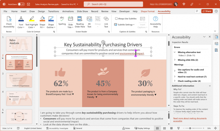
PowerPoint

Faster playback comes to Microsoft Stream videos

Microsoft Stream lets people in your organization upload, view, and share videos securely. You can share recordings of classes, meetings, presentations, training sessions, or other videos that your team needs. We previously enabled Stream as one of the supported online video sources in PowerPoint. Over the last few months, we’ve made significant performance improvements to the video playback experience. Now you’ll experience faster playback of Stream videos in your PowerPoint presentations.

Outlook

Create polls in email quickly and easily

Easily create a poll, collect votes, and view results within an email.

Learn more>

Quickly reopen items from previous session

We added an option to quickly reopen items from a previous Outlook session. Whether Outlook crashes or you close it, you’ll now be able to quickly relaunch items when you reopen the app. This feature is on by default. To turn it off, go to Options > General > Start up Options.

Learn more>

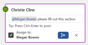
Disable @ mentions

Do you find the @ mention picker more annoying than useful? Now you can turn it off. Find the option under the new checkbox under File > Options > Mail > Send Messages in Outlook.

Transfer Outlook settings automatically

Outlook will now store/retrieve settings from the cloud, so when you set up a new Windows device, your settings will be loaded automatically based on your Office identity.

Store your signatures in the cloud

Signatures now follow your account across Windows devices. Set up your account once, and new installations of Outlook will have your signatures.

July 17, 2020

Excel

Notables fixes

We fixed an issue where any time a pivot chart with hidden leader lines was saved and reopened, the leader lines would become visible.
We fixed an issue where charts were not always updated as expected when “ForceFullCalculation” was enabled via VBA for the workbook.

Word

Notable fixes

We fixed an issue where the Show Markup command was disabled when the focus was on a comment text box.
We fixed an issue where the Editor command was disabled when the focus was on a comment text box.
We fixed an issue in custom XML that state of comments may be lost when opening the document.

Outlook

Notable fixes

We fixed an issue around creating multiple profiles in Outlook from the same email domain.
We fixed an issue that caused the lock icon to fail to display in the header of S/MIME encrypted messages.
We fixed an issue that caused attachments to get stripped from S/MIME messages when sending as unencrypted.
We fixed an issue that caused users to be unable to save OneDrive attachments from outside their tenant to their local computer when selecting the Save option on the security dialog.
We fixed an issue that cause recipients to be unable to save rights protected messages even when the save as permission was granted by the sender.
We fixed an issue that caused plain text S/MIME messages to become garbled when sending.
We fixed an issue that caused attachments to become corrupted when sending an S/MIME email unencrypted.
We fixed an issue that caused the labels for some Advanced Search options to be truncated in some languages.

Project

Notable fixes

We fixed an issue where the tasks listed in the Task Board view were not in sync with those in the Assign Resources dialog.
We fixed an issue where if you copied and pasted a task that had multiple dependencies, not all dependencies were copied correctly.

Office

Notable fixes

We fixed an issue where after the user opened a new app window from the taskbar and created a new blank document, additional files were created.
We fixed an issue where if a user was editing a document but had lost permissions, we were not notifying the user that they had to re-authenticate.

July 24, 2020

Visio

Create charts with data in worksheet

Visio Data Visualizer can help users convert their excel data into high quality flowcharts, swim line diagrams, and org charts. These diagrams can be viewed in Visio, downloaded as images, printed, etc. They can also be opened in Visio for richer editing capabilities.

Learn more >

Word

Notable fixes

We fixed an issue where an occasional hang occurred while opening HTML files.
We fixed an issue where the Specific People option for Track Changes was disabled.
We fixed an issue where the placeholder text in the Search edit box would overflow if the application window was resized to a small dimension.

OneNote

Notable fixes

We fixed an issue where the placeholder text in the Search edit box would overflow if the application window was resized to a small dimension.

July 31, 2020

Excel, PowerPoint, Word and Outlook

Insert Apple photos into Office easily

We’re happy to announce inserting Apple photos into Office is easier than ever. You can now insert pictures taken with your iPhone or iPad into Word, Excel, PowerPoint, and Outlook on Windows! We had heard from many of you that converting these files was too time consuming, so we’ve simplified the process.

Learn more >

Excel, PowerPoint, Word

Notable fixes

We fixed an issue where a copy of an image with a radial gradient fill did not match the original.

Excel

Notable fixes

We fixed an issue where if the order of a chart series was changed, the corresponding checkbox aligned with the series was not reordered along with the series.

PowerPoint

Notable fixes

We fixed an issue where the Forms button in PowerPoint did not allow the creation of Forms when access to the Office Store was not permitted.

Word

Notable fixes

We fixed an issue where if a comment was added to track a change, the revisions pane would unexpectedly open.
We fixed an issue where links to documents were not being inserted to the comments box via the Insert > Link dropdown.
We fixed an issue where the hyperlink count in the VBA hyperlinks collection was not iterating correctly after adding an image containing a hyperlink.

Outlook

Notable fixes

We fixed an issue that caused users to be unable to add a signature when replying to a digitally rights managed message from an inspector window when the user did not have Owner permissions on the message being replied to.
We fixed an issue that was causing Outlook to fail to display line breaks properly in markdown content.

Access

Notable fixes

We fixed an issue where trying to run certain queries have previously produced the error message “Query is too complex.”

Project

Notable fixes

We fixed an issue where for a SharePoint tasks list, the ribbon buttons on the second tab may be disabled.

We compiled all the new features and fixes in July in Office insider. Hope to see you in our other articles, bye bye. 🙋🏻‍♂️

You can share this article with your friends and family to help them get information about Office insider updates released in the month of July. 👍🏻

file trickster office insider Office365

Office Insider – What happened in August?

NEW FEATURES/FIXES

📅August 07, 2020

PowerPoint

Notable fixes

We fixed an issue where users were seeing the ribbon/title bar not being displayed under certain conditions.

Outlook

Notable fixes

We fixed an issue where the user account attributes in Active Directory for “otherTelephone” and “otherHomePhone” were not mapped to the corresponding Outlook LDAP attributes.

📅August 11, 2020

Word

Explore modern comments

Add comments to objects, @mention colleagues, and resolve comment threads for a better collaboration experience.

Word’de modern açıklama ekleme

Learn more >

Outlook

Delete messages

Delete messages and conversations in CML view.

📅August 14, 2020

Excel

Notable fixes

We fixed an issue where if a user typed a formula name including the parenthesis and invoked help via F1, the help topic specific to that formula would not be displayed.
We fixed an issue where macro links to buttons were broken after restoring the file to an older version of Excel.

Word

Notable fixes

We fixed an issue where the bullet picture icon didn’t display correctly.

Outlook

Notable fixes

We fixed an issue where the Meeting page would continue to be displayed after the user switched tabs from the Meeting page to the Scheduling Assistant page.

We compiled all the new features and fixes in August in Office insider. Hope to see you in our other articles, bye bye. 🙋🏻‍♂️

You can share this article with your friends and family to help them get information about Office insider updates released in the month of August. 👍🏻

file trickster office insider Office365

The RANDARRAY Function

In this article, I will be talking about one of the new dynamic array functions: the RANDARRAY function. Sometimes we need a data table filled out with random data. With this function, you can quickly fill as many rows and columns with numeral data. And you can find our articles about other functions on our blog.

WHAT DOES IT DO

The RANDARRAY function returns an array of random numbers. You can specify the number of rows and columns to fill, minimum and maximum values, and whether to return whole numbers or decimal values. The function returns a random set of values between 0 and 1 if you don’t enter an argument. For example, you can create a 20-row and 5-column table that contains whole numbers between 50 and 500 quickly in a few seconds.You will see an example below.

SYNTAX

=RANDARRAY([rows],[columns],[min],[max],[whole_number])This function has 5 arguments.
All of them are optional.

Now, let’s take a look at these arguments and what they mean, and what we will give them.

[rows]

Optional

The number of rows to be returned

[columns]

Optional

The number of columns to be returned

[min]

Optional

The minimum number you would like returned

[max]

Optional

The maximum number you would like returned

[whole_number]

Optional

Return a whole number or a decimal value

TRUE for a whole number
FALSE for a decimal number.

WORKING CONDITIONS

If you don’t input a row or column argument, RANDARRAY will return a single value between 0 and 1.
If you don’t input a minimum or maximum value argument, RANDARRAY will default to 0 and 1 respectively.
The minimum number argument must be less than the maximum number, otherwise RANDARRAY will return a #VALUE! error.
If you don’t input a whole_number argument, RANDARRY will default to FALSE, or decimal value.
The RANDARRAY function will return an array, which will spill if it’s the final result of a formula. This means that Excel will dynamically create the appropriate sized array range when you press ENTER. If your supporting data is in an Excel table, then the array will automatically resize as you add or remove data from your array range if you’re using structured references. For more details, see this article on spilled array behavior.
RANDARRAY is different from the RANDfunction in that RAND does not return an array, so RAND would need to be copied to the entire range.
An array can be thought of as a row of values, a column of values, or a combination of rows and columns of values. In the example above, the array for our RANDARRAY formula is range D2:F6,or 5 rows by 3 columns.
Excel has limited support for dynamic arrays between workbooks, and this scenario is only supported when both workbooks are open. If you close the source workbook, any linked dynamic array formulas will return a #REF! error when they are refreshed.

USE OF THE FUNCTION

Now, let’s see how this function works with 3 different examples. First, we will determine rows and columns. And then we will give row, column, min and max number values and return a retrospective array. And then, we will request the numbers to be returned to be whole number. The image we will obtain is going be like this:

See you in other articles, bye. 🙋🏻‍♂️
You can share this post with your friends and get them informed as well. 👍🏻

Excel file trickster msexce office insider RANDARRAY rasgdizi

Office Insider – What Happened in March?

NEW FEATURES/FIXES

March 28, 2020

Outlook

Calendar visual refresh

Last year, we brought you a refreshed mail experience, and, this year, it is the calendar’s turn to get a facelift! The updates are fresh but familiar so, as a seasoned Outlook user, you can jump in and be more productive right away.

Learn more.

Takvimde çalışma haftasının resmi.

Notable Fixes

This change addresses delays when processing images with malformed or invalid protocol information.
This change fixes an issue where the latest changes to draft emails were not being updated.
Fixed an issue where right-mouse clicking on a file and using ‘Send to’ would not work.
Fixed an issue where if a user had a customized the search path for the Address book, Outlook’s name resolution scope would be limited to the customized path rather than including the Global Address List (GAL).
Fixed an issue where within a set of returned search results, sorting the results by Categories would not display the Category colors.

PowerPoint

Synchronize changes while you are presenting

For years, PowerPoint didn’t allow changes made to slides by others to be displayed while presenting. This ensured that the presenter was in full control of the content being shared. No one could revise slides, either accidentally or maliciously. It also ensured that all of your computer resources were used for slideshow rendering. A concern that is especially important if you are running on a low-end machine.

However, while some presenters may still desire this original design, we’ve heard from others that they are seeking more flexibility. With an increased focus on collaboration and real-time updates, we’re excited to make available the ability to synchronize changes whenever they are made, even when the presentation is in Slide Show mode.

How it works

You can synchronize changes in two ways: automatically or manually.

Automatically update slide content

1. Select the Keep Slide Updated check box on the Slide Show tab on the ribbon.

PowerPoint

2. Start the presentation by selecting the appropriate button on the Slide Show tab.

3. Whenever an update to a slide is made and detected, the content is automatically updated and visible in the slide show being presented.

Manually update slide content

1. Clear the Keep Slide Updated check box on the Slide Show tab on the ribbon.

2. Start the presentation by selecting the appropriate button on the Slide Show tab.

3. Whenever an update to a slide is made and detected, an Update Slides button appears at the top of Presenter View.

4. Click the Update Slides button to manually synchronize the slide content.

Word

Notable Fixes

Fixed an issue where the functionality to post comments was disabled.
This change addresses delays when processing images with malformed or invalid protocol information.
This change addresses an issue where the account manager would not dispatch messages resulting in a hang with third party applications.
This change fixes an issue where the Table of Contents would get updated with heading styles which were not present in the document.
Fixed an issue where digital signatures saved in Word documents would be removed when mailing the documents.

Excel

Notable Fixes

This change addresses delays when processing images with malformed or invalid protocol information.

Project

Notable fixes

Fixed an issue where the ‘ProjectBeforeTaskChange’ Visual Basic Applications (VBA) event did not fire when a user clicked the “Inactivate” button found on the Tasks Ribbon within the Scheduling grouping.
If you set predecessor or successor details from within a Form type view, the ProjectBeforeTaskChange Visual Basic Applications (VBA) event didn’t always capture the changes. For example, if you deleted a dependency and clicked OK on the form, the event did not fire. This behavior has been fixed.
Fixed an issue where the latest values for the Actual Cost of Work Performed (ACWP) would not be displayed after making a change, such as a date change.
Fixed an issue where opening a project using the Most Recently Used (MRU) menu opened the project file with Read/Write access.
This change fixes an issue where if you created a manual task with a start date and a time (but no duration), it would be displayed with an incorrect time on the timeline.
Fixed an issue where printing a timeline using Hijri calendar would result in a month being skipped or duplicated in the print view.
This change addresses an issue where working in Team Planner with GDI objects, could result in the over allocation of GDI objects and create low memory conditions.

March 13, 2020

Word, Excel,PowerPoint andOutlook

Sensitivity labels

You can now apply a sensitivity label that your organization has configured to prompt you for custom permissions. Learn more

How to Access

If your organization has set up Sensitivity tags in Microsoft Information Protection and enabled users to assign permissions, you can access them. For example, choose Home> Protect, then select the label you want to apply to the document, workbook, presentation, or email.

İzinlere nasıl erişileceğini gösteren Word belgesinin resmi.

Outlook

Notable Fixes

Addresses an issue that caused the “Last Modified”; date on a file to be updated when adding an attachment to a mail or saving an attachment from a mail by dragging and dropping it (as opposed to via a menu).
Addresses an issue that caused hitting enter in the expanded find pane to fail to start a search, requiring instead that users click on the search button.
Fixed an issue where search shows no information about users when the option to “Show user photographs when available” is disabled.

Word

Notable Fixes

Fixed an issue when typing or editing a comment and using Ctrl+A would result in selecting text in the canvas instead of selecting text just within the comment card.
We fixed an issue in which the alignment of words in a document gets scrambled when tried to edit after printing using Quick Print.
We fixed an issue when merging two documents into one document.
Fixed an issue where marking revisions involving equations could result in a failure when saving the file.

Excel

Notable Fixes

Fixed a performance issue that users may have experienced when programmatically editing a large range of cells.
Fixed a performance issue that occurred when opening csv files with Japanese environments.

Project

Notable Fixes

Fixed an issue where summary task dates weren’t always getting calculated correctly.
Fixed an issue where the OnUndoOrRedo event doesn’t fire without first running the OpenUndoTransaction method.

Access

Notable Fixes

Fixed an issue where international versions of Access were displaying English strings in the user interface.

PowerPoint

New Features

Look above.

March 10, 2020

Excel,Word,PowerPoint andOutlook

Pick the perfect color

We heard you! Converting Hex colors to RGB values is now a thing of the past. For any property where you can define a color, click the appropriate button in the ribbon (such as the Font Color button) and click More Colors. Then, in the Colors dialog box, click the Custom tab and enter the Hex color value in the Hex box, for example, #0F4C81 or 444.

Learn more

Onaltılık bilgiler alanını gösteren renkli kutu.

Excel

Automatically use new data types*

When you type a data value that resembles a possible stock or geographic location, Excel offers to convert it to the appropriate connected data type – Stocks or Geography. Give it a try!

Type in several geographic locations (such as “Seattle”, “London”, or “Tel Aviv”) or stock ticker symbols (such as “MSFT”, “ADBE”, or “AAPL”) in separate cells in a column.

When Convert to Geography or Convert to Stocks appears to the right of the selected cell, click on it.

Verileri dönüştür kutusunun bulunduğu Excel çalışma kitabı.

* This feature is only available in English right now.

Outlook

Drag emails to a group you own

As a group owner, you can now move and copy messages and threads by dragging and dropping them from your mailbox to the groups’ mailbox. Once moved, the content is visible to all the group members, and anyone can read the messages and participate in the conversation.

Learn more

Better search results, faster

The Search experience in Outlook just got a facelift! It is now more reliable, intelligent, and faster than ever. Also, any search entry is now being spell checked and, if errors are detected, helpful suggestions are offered to ensure that you get to the results you’re looking for. Finally, notice that the most relevant search results are presented at the top of the results list, making access faster.

Arama öğelerinin vurgulandığı Outlook posta kutusu resmi.

PowerPoint

Diagrams get connector support

Now, the converted lines between objects are connectors anchored to the shapes.

Ink conversion is also easier than ever with just clicking the Convert your ink button . Select the converted object again to be able to access other conversion alternates, to make sure the conversion fits your needs. Give it a try! Give it a try!

Sağda siyah bağlayıcı dönüştürme kutusuyla boş beyaz kutular.

March 6, 2020

Outlook

Notable fixes

We fixed an issue that was preventing users from attaching a file to their mail messages when that file was open in another application.
We fixed an issue where creating a rule with Outlook Web Access did not persist to the Exchange server and resulted in a conflict.
We fixed an issue with Outlook that wouldn’t show the drop-down list in the “From” field when using dark mode.

Word

Notable fixes

We fixed an issue that made the User Principal Name (UPN) people case-sensitive, e.g., [email protected] would fail to match [email protected], and prevented users from accessing the SharePoint Sites service.
We fixed an issue that prevented the Compare feature from working when the document was protected for editing.

PowerPoint

Notable fixes

We fixed an issue that made the User Principal Name (UPN) people case-sensitive, e.g., [email protected] would fail to match [email protected], and prevented users from accessing the SharePoint Sites service.
We fixed an issue where the recommended thumbnails flashed when hovering your mouse over the thumbnails. In some cases, this could cause PowerPoint to crash.

Excel

Notable fixes

We fixed an issue that made the User Principal Name (UPN) people case-sensitive, e.g., [email protected] would fail to match [email protected], and prevented users from accessing the SharePoint Sites service.

We compiled all the new features and fixes in March in Office insider. Hope to see you in our other articles, bye bye. 🙋🏻‍♂️

You can share this article with your friends and family to help them get information about Office insider updates released in the month of March. 👍🏻

file trickster O365 offfice 365 office insider Office365