Tag: file trickster

Sort and Fill Data with Custom Lists

In this article, we will be talking about how to create a custom list in Excel and what we can do with it. We can get faster in entering and analyzing data by creating data tables quickly with custom lists. If you already have a data list, i.e. certain product names, brands, stock names, region names etc.; if you add them to custom lists once, it is possible to list all the data in the list quickly instead of writing them over and over again. You just need to write any data from that list into a cell and drag it down. In addition, you can find articles concerning other features of Excel on our blog.

HOW ARE THE CUSTOM LISTS STORED?

Once you create a custom list, it is added to your computer registry, so that it is available for use in other workbooks. If you use a custom list when sorting data, it is also saved with the workbook, so that it can be used on other computers, including servers where your workbook might be published to Excel Services and you want to rely on the custom list for a sort.

However, if you open the workbook on another computer or server, you do not see the custom list that is stored in the workbook file in the Custom Lists popup window that is available from Excel Options, only from the Order column of the Sort dialog box. The custom list that is stored in the workbook file is also not immediately available for the Fill command.

If you prefer, add the custom list that is stored in the workbook file to the registry of the other computer or server and make it available from the Custom Lists popup window in Excel Options. From the Sort popup window, in the Order column, select Custom Lists to display the Custom Lists popup window, then select the custom list, and then click Add.

HOW ARE CUSTOM LISTS CREATED?

You need to access the existing custom lists box to create a custom list. There are two ways to access that box.

File > Options > Advanced > Edit Custom Lists

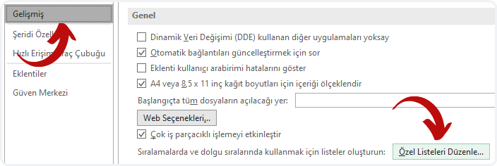
2. Data > Sort > Order > Custom Lists

BUILT-IN LISTS

Excel provides day-of-the-week and month-of-the year built-in lists. The names will change depending on the language you use.

Built-in lists
Sun, Mon, Tue, Wed, Thu, Fri, Sat
Sunday, Monday, Tuesday, Wednesday, Thursday, Friday, Saturday
Jan, Feb, Mar, Apr, May, Jun, Jul, Aug, Sep, Oct, Nov, Dec
January, February, March, April, May, June, July, August, September, October, November, December

Note: You cannot edit or delete a built-in list.

For this reason, when we type January into a list and drag it down, a list that goes like February, March, April is created. If these lists didn’t exist, when we dragged the list it would have gone like January, January, January.

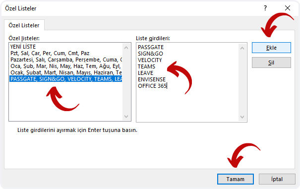
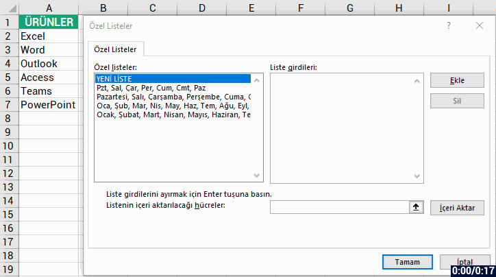
HOW DO YOU CREATE A CUSTOM LIST MANUALLY?

Access the Custom Lists Box with one of they ways we’ve mentioned above.
Enter the data you want into the List entries field.
Click Add.
You will see that it is added in the Custom Lists field.
Finally, click the OK button.

Now you will see that when you write and drag any data that you’ve entered to the List entries field, every single one of them will be listed.

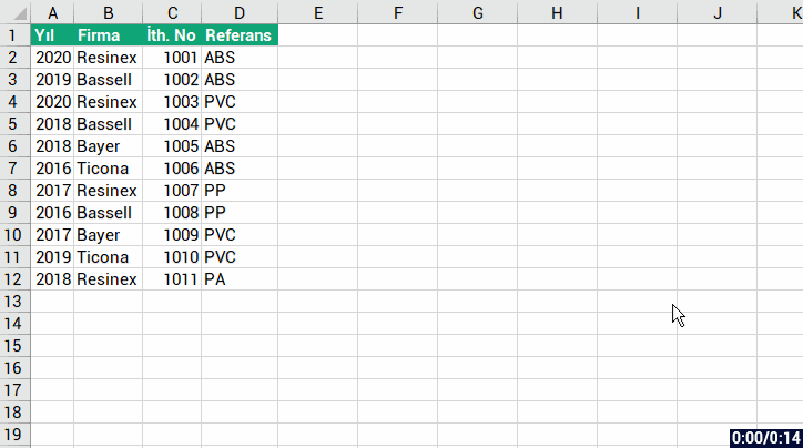
Let’s quickly create a data table that contains of the data we created and also months.

IMPORT YOUR DATA TO YOUR CUSTOM LISTS

If you have steady and unique data in a range of cells, you can import that date to the customs listens box as a whole and use them in your lists. For that you need to go to the Custom Lists box from File > Options > Advanced > Edit Custom Lists. Afterwards, we will select the cell range and import the content.

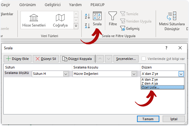
And the thing about accessing these lists from the Sort window is that you can use them with the Sort feature.

For example; there are multiple lists in a table and you want to sort the list but you want 2019 and 2020 be the primary ones. You can add the 2019 and 2020 data into the Lists box and sort the way below.

You can get detailed information on Office Support.

See you in other articles, bye. 🙋🏻‍♂️
You can share this post with your friends and make sure that they are informed too.👍🏻

Create Custom Rules in Conditional Formatting

I will be talking a bit about how you can create custom rules for conditional formatting. Of course, to be able to create these rules, you need to be able to write formulas, at least a bit. I will tell you about how to create simple formulas and use them in conditional formatting. As you get better at writing formulas, I am sure that you will create better rules. You can take a look at our blog to find other articles about the other features.

WHAT IS CONDITIONAL FORMATTING?

One of the most frequently used features in Excel is Conditional Formatting. This feature is usually used to color and highlight backgrounds of certain cells that comply with a specific rule. It is found within Styles in the Home menu. There are some available rules you can use. When the available rules are not enough for you, you can create your own rules and format the cell in compliance with those rules. Of course, for this you need to know how to write formulas like I have mentioned above.

We can see the available prepared rules when we choose Conditional Formatting like you can see below. We can easily format by color, text, and date. If the available rules are not enough for you, then you can choose “Use a formula to determine which cells to format” from the New Rule option and highlight the cells that comply with your rules by writing to the formula into the related field. If we want, we can create more than one Conditional Formatting in a field. We can use the Manage Rules option to see and change the conditions of these formats.

You can use the Clear Rules option to clear rules in a part of the page or in the whole page.

Let’s dig a bit deeper with practical examples.

APPLY CUSTOM RULES IN CONDITIONAL FORMATTING

HIGHLIGHT TEXTS

In our first example, we will make a simple application about creating custom rules in conditional formatting. Let’s detect and highlight backgrounds of texts in the field we determine. For this, we need a function that would detect if a value in a cell is text or not. This function is called: ISTEXT. We will be able to automatically highlight the data if they are text in the specified field.

You can see how to do it in this GIF and do the same thing for your work.

HIGHLIGHT WEEKENDS

Let’s detect the weekends of the dates in a columns and highlight their backgrounds for our second example. We will need a function for this as well, and it is called WEEKDAY. With this function, we can find out which day a date is in its week. I.e, it will give us a number between 1 and 7; and we will highlight the dates that happen to be weekends by writing a rule of if the number is bigger than 5.

First, I want to do a live application of this formula for you to do it live as well and comprehend it better. After writing the formula to the cell, we will copy that formula and paste it to the use formula section in conditional formatting.

And as the last step, we will write this formula to the related field, click on format and complete the action.

If you say that you need more information, you can check Office Support.

See you in other articles, bye. 🙋🏻‍♂️
You can share this post with your friends and enable them to get informed as well.👍🏻

conditional formatting Excel file trickster kural oluşturma msexcel

How to Make a Histogram in Excel

In this article, we will be talking about how to make a histogram in Excel. It looks a lot like the other bar charts, but separates your numbers into ranges the way you determine. Compared to the other chart types, histograms facilitate determining categories and frequencies of occurrence alongside different data. Don’t forget that you can take a look at our blog to see our articles about other topics. Let’s start. 👍🏻

HISTOGRAM IN EXCEL

You can find the Histogram Chart within built-in charts in Office 2016 and later version. Also, you can create a histogram in Excel with the Histogram tool. You create it by entering the numbers that represent the frequency range you want to use and the data you want to analyze. Histograms are supported by Office 365, Excel 2019, 2016, 2013, 2010, 2007 and Excel for Mac, but the steps you take depend on the Excel version you use.

Reminder: You need the Analysis ToolPak extension to use the Histogram tool in the previous versions of Excel 2016. This extension is not supported in Excel Online. But, you can display a histogram created in a desktop version of Excel by using Excel Online.

How Do You Create a Histogram Chart in Excel?

Since it is one one the built-in charts in Excel 2016 and later versions, it is pretty easy to use.

To start, enter the data you want to use in your histogram into a worksheet. For example, enter the names of your employees in your company with 1000 workers into a column, and their ages into another column.
Select any cell on your data table.
Go to the Insert menu.
Choose Insert Statistic Chart in the charts group.
Choose Histogram chart type.
Double-click on the horizontal axis.
Arrange the bin width as 5.
Add Data labels.
Your chart is ready.

Creating a Histogram chart is as simple as that. If we want to apply the steps above, a Histogram chart like this will come up. (The colors have been edited.)

Let me show you how the steps are done with a GIF:

Creating a Histogram in Excel 2013, 2010 or 2007

Like I mentioned above, you need to active the Analysis ToolPak extension to be able to create a histogram chart in versions prior to 2016.

Click the File menu.
Choose Options.
Click on Extensions.
Push the Go button.
Choose the Analysis ToolPak extension.
Click on the OK button.

After following these instructions, you will see the Analysis ToolPak extension within the Analysis group on the right of the Data menu. We will show you how to activate it on the GIF below.

To get a Histogram from the Analysis tool, let’s write the bin width into a field first. For example; let’s write the bins starting from D2 as 28, 33, 38, 43, 48 to find how many people there are between the ages of 23 and 48 with 5 year gaps in a company with 1000 employees. You can check the GIF below for the next step.

HINT: We can obtain the same Histogram that comes with data analyzes with the FREQUENCY function. We have data, and certain tracking ranges. With the FREQUENCY function, we can easily find the frequency of repetition of all values within the specified range.

You can find chart and application samples about everything I’ve mentioned in this Excel file. 👉🏻

You can get more information on Microsoft Support.

See your in another article, good bye.🙋🏻‍♂️
You can share this post with your friends and help them get informed as well.👍🏻

ecel histogram Excel excel grafik file trickster histogram histogram grafik msexcel

Get a Picture from a Cell with a Formula

In this article, I want to explain you how to get a picture to a cell with a formula. As you know, we can get the data of the columns we want from a table by looking up for a value on the specified table with lookup and reference functions like VLOOKUP but we can only get the data inside a cell. At this point, what we want to tell you is that if there is a picture in the are we want to get, we can get it with a formula. By the way, we would like you to read and analyze our articles about Office, you can find them on our blog.

Get a Picture to the Cell with a Formula

Let’s say that we have two different pages. On one page, there are products, brand names etc. and on the other page there are product and brand pictures. We can get the picture on the second page next to the product and brand name on the first page with a formula that we’ll write. While doing that, as you’ll see below, we need to define names. We cannot get the picture in a cell without defining names.

Here is how you do it step by step:

Create a Data Verification list with brands.
Write the main formula necessary for this action.
Name the formula we created with the Name Manager.
Complete the process by assigning the name to the picture.

Let’s start understanding how to do it with pictures! 😀

We talked about creating a data verification list first, let’s take a look at it.

We took the brand names to the data verification list.Let’s write the formulas that will do the job. I am leaving the formula here, you can see how I write it in the gif below.

=İNDİS('6-1'!$B$2:$B$6;KAÇINCI('6'!$A$2;'6-1'!$A$2:$A$6;0))

Now we’ll name the formula I have written, assign the picture on the first page and complete this action.

As you can see, we have learned how to get a picture to a cell with a few steps.. We have called a picture on another page to the active page with brand names. You can execute this kind of examples by getting pictures dynamically.

Also, you can get more information about defining names on Microsoft Support.

See you in other articles, bye.🙋🏻‍♂️
You can share this post with your friends and help them get informed. 👍🏻

ad tanımlama define name Excel Excel ad tanımlama excel formül Excel functions file trickster formülle resim getirme msexcel

Office Insider Program – How to Join

What is the Windows Insider Program?

Microsoft Insider

was created for all Microsoft 365 users.

Office insider participants are granted first-hand access to new features and updates.
You can access dynamic array formulas.
In addition to this, you can share your comments about developments with the developers.

Click here to become an Office Insider member.

Access to the Insider Program

The procedure below is the simplest and most complete one.
For a long time it was blocked to go back to “standard” Excel version after you became an Insider .

But with this method you can change between channels anytime you want.

When you go to File> Account menu and want to see information about Microsoft Account like synchronized files, you will see that there are 3 standard buttons that enable you to know your software version number and Office news. If you cannot see the Office Insider button there, follow the steps below.

1st Step: Add Office Insider Button to your Account

After yo do the settings below, you will see that the 4th button is added too. Click on the Insider button.
To do it you need to add a key into registry. To open your registry type regedit on your Windows taskbar.

Normally Office, 16.0 and Common arrays are not on registry, you need to create them.

Path : HKEY_CURRENT_USERSoftwarePoliciesMicrosoftOffice16.0Common
Key Name: insiderslabbehavior
Value type : REG_DWORD
Value : 1

After you restart Office you will see that on the File > Account menu you have the Office Insider button.

2nd Step: Changing Office Channel

Then, to see both of the recommended levels click on the Insider > Modification Level button.

You can see 2 levels of the available update by clicking on the popup menu: Monthly Channel or Insider.
Needless to say you need to accept terms of use to change the channel of your application.

3rd Step: Differences between the Two Programs

Insider Channel
This is the level that open the latest Office updates. Some of them didn’t have the chance to be tested by the developers or to be completed. Thus, it carries a risk to fail your Excel functions and collapse your workbooks (it is pretty common). However, it is the only way to access latest features like XLOOKUP.

My recommendation: Don’t set up this version on a professional environment. Would be better in a test machine.

Monthly Channel
This channel is not for test users, it is for very advanced level Excel users. This version opens up persistent features that are usually non-existent in Office standard version (six month channel). For example, to be able to use dynamic array functions you need to subscribe to one of the 2 levels of Insider. If not, you cannot use them.

For this, if some of your employees want to access features that require Insider, this channel is the one that needs to be set up.

4th Step: Update Office

Whatever Office level you choose, it is a must to update your Office.
Single selection of Office channel is not enough to open the Insider program.

After you choose one of the insider levels and click on update button, upgrade will start automatically.

5th Step: Restarting Excel

It is enough to restart your Office apps once or twice to see the changes.

Going back to the Six Month Channel (standard version)

The only thing you need to go back to the six month channel which is Office’s basic version:

Click on the Insider icon.
Uncheck Save to Preview new versions of Office option
Update Office again.

Don’t forget to check other articles on our blog.
You can share this article and make sure that many other people get informed as well.

Bye. 🙋🏻‍♂️

file trickster insider programı office insider

Office Insider – What Happened in June?

NEW FEATURES/FIXES

You can find and follow all monthly Office insider new features and fixes (updates) on our blog. 👍🏻 Officer insider gets updates and new features regularly. It is important to follow these Office insider updates and use them in terms of increasing your knowledge. Now let’s take a look at what kind of changes happened in Office insider in the month of June.

June 06, 2020

Excel

Sheet View

Now you can sort and filter your Excel file while collaborating with others with Sheet View.
Thanks to this new feature, users working on the file together don’t get affected by the others’ sorting and filters.

Create PivotTables from Datasets in Power BI

Now, you can create PivotTables connected to datasets stored in Power BI in Excel with just a few clicks. This allows you to get the best of both PivotTables and Power BI.
Calculate, summarize, and analyze your data with PivotTables from your secure Power BI datasets.

Learn More

Notable fixes

An issue that caused the custom values in the chart axis not to be applied correctly has been fixed.
An issue that caused saving worksheets containing multiple formulas with defined names to take more time compared to now.

Outlook

Quickly reopen items from previous session

We added an option to quickly reopen items from your previous session. Now you can automatically restore items that were open when Outlook got locked or closed.
To turn off the feature go to Options > General > Start up options.

önceki oturumdaki öğeleri yeniden açma

Notable Fixes

An issue where the Input Method Editor (IME) window would overlap the underlying text being entered via the IME when using multiple monitors with different resolutions has been fixed.
An issue where viewing a template when composing a new email message would result in a crash has been fixed.
An issue where users were unable to Exchange 2010 public folders after Outlook version 1911 has been fixed.
An issue where the Categorize button for group calendars in the Office Ribbon was disabled has been fixed.
An issue that caused users to experience a crash in Outlook when working with hyperlinks in plain text emails has been fixed.
An issue that caused Outlook to be unable to parse long file names encoded with RFC2231 has been fixed.
An issue that was causing Outlook users to experience intermittent hangs when using screen readers has been fixed.
An issue that resulted in the Online Archive dropdown in folder properties to be missing for users on high DPI monitors has been fixed.
An issue that would cause users with conflicting contacts to experience crashes in Outlook has been fixed.

Word

Notable fixes

An issue where timestamps in Comment panes were not based on the system locale time has been fixed.
An issue where comments between the web app and the desktop application were not in sync has been fixed.

PowerPoint

Notable Fixes

We fixed an issue where the slide editor from one slide would overlap on to the next slide.
We fixed an issue where a Comment pane that had been closed by the user would re-open automatically.
We fixed an issue where PowerPoint files with embedded charts/workbooks could result in failures when saving the file.
We fixed an issue with opening files from server-configured with Forms-based authentication.

Project

Notable Fixes

We fixed an issue that prevented orphaned tasks from being deleted or reassigned after the parent plan was deleted.

June 12, 2020

Excel

Get Organization Data from Power BI using Data Types

Excel data types from Power BI are now rolling out to Insiders in organizations with Office 365 E5/A5 or Microsoft 365 E5/A5. Getting the information you need and easily refreshing it is critical to many everyday workflows. You can access your company or organization information from Power BI as a data type in Excel, which expands your ability to bring in linked information in your spreadsheets.

Learn More

Notable Fixes

An issue where the major gridlines of radar charts could not be formatted correctly has been fixed.

Word

Notable Fixes

An issue where the ability to clear formatting within the Comments pane via the Clear Formatting button in the Office Ribbon was not working has been fixed.
An issue where changing the size of a table when the ruler is not displayed caused other applications running in the background to start flashing has been fixed.
An issue where if Word had a list of more than 50 frequently opened documents, then after saving and opening a document, a revision history would be displayed even though no revisions were made to that document has been fixed.

Project

Notable Fixes

An issue where a baseline reset or update could change time-phased budget cost/work resources and the baseline could reflect incorrect budget values has been fixed.
An issue where the ProjectBeforeTaskChange event didn’t fire when there was a change to the project summary task, either the project start/task field has been fixed.

Access

Notable Fixes

An issue that caused Microsoft Access to fail to identify an Identity Column in a linked SQL Server table, which could cause rows to be reported as deleted incorrectly has been fixed.

June 19, 2020

Excel

Notable Fixes

An issue where workbooks were read-only when the file only had read-only recommended has been fixed.
An issue where CustomUI XML for a custom ribbon tab was removed when saving to SharePoint /OneDrive has been fixed.

PowerPoint

Notable Fixes

An issue where a user’s presence color indicator was not getting refreshed in the co-authoring gallery during a live, co-authoring session has been fixed.

Word

Notable Fixes

An issue where the HTML hyperlink color was not being rendered correctly has been fixed.

Outlook

Notable Fixes

An issue where the Input Method Editor window would overlap the underlying text being entered via the IME when using multiple monitors with different resolutions has been fixed.
An issue where the dates in mini calendar failed to display in bold for users in Japan has been fixed.
An issue that prevented calendar reminders from showing exact times for the meetings coming up in less than a week has been fixed.
An issue that caused users to see the following error when closing an appointment that was previously saved has been fixed: “The item cannot be saved because it was changed by another user or in another window. Do you want to make a copy in the default folder for the item?”

Project

Notable Fixes

An issue where if Fixed Duration tasks are%100 complete but Actual Finish is not specified, the Task % Complete would display as less than 100% has been fixed.

Office Suite

Notable Fixes

An issue where the URLs that were not http or http based were not being displayed in the Most Recently Used list hast been fixed.

We compiled all the new features and fixes in June in Office insider. Hope to see you in our other articles, bye bye. 🙋🏻‍♂️

You can share this article with your friends and family to help them get information about Office insider updates released in the month of June. 👍🏻

file trickster office insider Office365