The Weekday Function

In this article, I will be talking about on of the Date and Hour functions, the WEEKDAY Function that will helps us in our daily lives. This function returns the number that represents the day of the week of a specific date. It gives us a number between 1 and 7, and so we know which day of the week it is and do actions depending on that. If you want, you can get the details about the Weekday Function on support office. You can find our articles about the other function on our blog


WHAT DOES THE WEEKDAY FUNCTION DO?

The WEEKDAY Function

gives us a number stating the which day a date is in that week. For example, If we want to know which dates in a column are weekend, we can have them highlighted. Or, doesn’t matter which day the payment days are in the column, if your payment day is Friday you can organize all the dates on Friday in their weeks.

SYNTAX

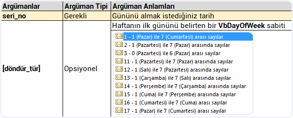
WEEKDAY(serial_number,[return_type])

The WEEKDAY Function

has 2 arguments.
The first one of them is required and the other one is optional.

Now let’s take a look at the meaning of these arguments, i.e. what this function wants from us and what we will give it.

haftanıngünü fonksiyonu argüman listesi


WORKING CONDITIONS

The working conditions of the WEEKDAY function are:

  • Microsoft Excel stores dates as sequential serial numbers so they can be used in calculations. By default, January 1, 1900 is serial number 1, and January 1, 2008 is serial number 39448 because it is 39,448 days after January 1, 1900.
  • If serial_number is out of range for the current date base value, a #NUM! error is returned.

  • If return_type is out of the range specified in the table above, a #NUM! error is returned.

  • If the Calendar is Gregorian, the returned number represents the Gregorian day of the week.
    If the calendar is Hegira, the returned number represents the Hegira day of the week. If the calendar is Hegira Calendar,  the argument number is any number that can represent a date and/or time from 1/1/100 (Gregorian Aug 2, 718) to 4/3/9666 (Gregorian Dec 31, 9999).


USING THE WEEKDAY FUNCTION

In the Weekday Function, we choose the date that we want to get the day number for the Serial_number argument first. Then, we choose the type that we want the Return_type argument to return. We will come across the list where the first and last days of the week are stated. For us the option is the one with the number 2, where first day is Monday and the 7th day is Sunday. So, we choose the 2 option for the return_type argument and complete the formula.


 HIGHLIGHTING THE WEEKENDS

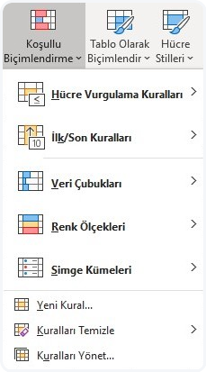
Let’s assume a list in which there are dates of March in a column. At the first glance, we cannot know which day those dates are. If you choose that column, choose Long Date as Format in the Number group in Home menu, you will get the day name and it might be useful for you. But we don’t want the day name, we want the weekends to be highlighted. We can achieve this with the WEEKDAY Function in the Conditional Formatting feature. Colors are very useful when it comes to analyzing a data.

Let’s start practicing with examples. You can apply these steps with me.
Unfortunately, an available rule that does what we want doesn’t exist in Conditional Formatting.
So, what do we do? We create our own rules with a formula, and achieve highlights based on that rule.
You can find and highlight the weekends like this.

weekday fonksiyon kullanımı


SETTING THE PAYMENT DAY AS FRIDAY

Let’s do an example of setting the payment day as Friday.
For this action, we will use the CHOOSE and WEEKDAY functions together.
Try to do this action as well and try to comprehend its logic by repeating few times.

weekday ile ödeme gününü cuma gününe ayarlama


See you in other articles, bye. 🙋🏻‍♂️
You can share this post with your friends and get them informed as well. 👍🏻

Methods of Declaring VBA Variables

In this article, we will be talking about Declaring VBA Variables. Variables are essential elements of programming. Using and managing variables are one of the musts while creating a project. I will try my best to tell it as simple as possible. Reminder: You can find other articles about VBA on our blog. 👍🏻


About Declaring VBA Variables

Variables are usually used to store a data and use it when necessary. They are usually separated into two classes. Global variables and Local variables. Global variables can be used by all the functions of the program, but the local variables are used by the functions that have declared them.

It can be called back, reassigned or fixed during the execution of a procedure, function or module.
Declaring a variable will enable you to indicate the names of the variable you’ll use and the data type the variable will contain.

For example, if Result = 10, the variable Result can be declared as Integer Whole Number .

We usually name the variables in a short and easily remembered way. The most frequently used variable names are one character names like i, a, n, x ,y ,z, s so that it is easy to write in the code. If the variable name is a name that you can remember while using in the code, the probability of making a mistake while writing the code decreases.

Now we can move on to the declaring part.


The syntax concerning declaring variables is usually like this.
Dim variable_name [(stringsize)] As type
Public variable_name[(stringsize)] As type
Static variable_name[(stringsize)] As type


Along side this general declaring, the declaring methods below can be used as well.

  1. Declaring with Dim
  2. Declaring with Data Indicators (Abbreviations)
  3. Declaring with DEF

Declaring with Dim

It is the most known and used VBA Variable Declaring method.

We indicated the syntax Syntax below. Let’s make it clear with a few examples. Let’s say that we will declare a variable named row to use in the rows (cells) in the A column. Since the row numbers are whole numbers, we can used one of the whole number types we’ve indicated in our Data Types article. It would be better to use the variable data type depending on the row number we’ll get controlled or the maximum number that can be in the cell.

As well as we can use as Number or Whole Number, we have 3 basic variable data types: ByteInteger and Long. If the number we’ll assign to the row variable is 255 or less, then we can use the Byte variable data type. If the number we’ll assign to the row variable is between –32767 and+32768, then we can use the Integer variable data type. If it can be a bigger whole number, then we should use the Long variable data type. If a bigger number than what the variable can contain is sent, that the Overflow error occurs. And if a text data is sent to a variable that was determined as number, Type Mismatch error occurs.


Let’s give a few examples of declaring variables with Dim:

Sub PEAKUP()
    Dim row As Long
    Dim column As Byte
    Dim text As String
    Dim start As Date
    Dim money As Currency
    Dim object As Object
    row = 15
    column = 5
    text = "Excel Turkey Forum"
    start = "24.06.2018"
    money = 300
    Set object= ActiveSheet
End Sub

We can write each variable one by one in different rows like that, but we also can write them side by side like this. We just need to put Dim in the beginning and put a comma between each variable.

Sub PEAKUP()
    Dim row As Long, column As Byte, text As String
    Dim start As Date, money As Currency, object As Object
End Sub

We need to be careful about this here: Some users make a mistake and declare incorrectly.

If you write the code I gave above like this one below, I mean if you start with Dim and think that you’ve declared the first variable and not declare the other variables with the suitable variable data types. Since in the “column”, “text” variable the data type is not stated, Byte and String are not indicated but Variant is -which is undefined data type. Since in the first variable I’ve declared with Dim, you declare the data type in the first variable. So, it doesn’t mean that you declare the next variables as well. You need to state the data type of each variable one by one.


Declaring with Data Identifiers (Abbreviations)

Abbreviations 

They are also known as Type Indication suffixes.
They are not used much but they help to save in codes.
It is also possible to tell a variable type by adding a special character to the end of the variable name in VBA.

Dim number% 'Integer
Dim longnumber& 'Long
Dim sum! 'Single
Dim subtotal# 'Double
Dim payment@ 'Currency
Dim name$ 'String
Dim longestnumber^ ' 64 bit LongLong


Data Type Abbreviation Characters

VBA

, as a fast way of declaring data type, lets you add a character in the name of a variable.
This method shouldn’t be used to declare variables and it can be used for retrospective purposes only.
The row below will declare a Double data type and a variable.

Dim dDouble#

But it is better for this row to be declared with the “As” keyword.
Dim dDouble As Double


Data Type Abbreviation/ Suffixes

If you you abbreviations, you don’t have to declare the type.
If you use the % expression, you don’t need to write “As Integer”.
These abbreviations can be helpful to get available information to Variants.

For example: count =10#


Declaring with DEF

We can declare our variables with different methods like we mentioned, one of these methods is declaring with DEF.
This declaration is usually done free from the procedure at the top of the code window.
We can abbreviate and declare the data type we use as variable like below.
The letter that comes after Def+Type indicated that the variables starting with that letter belong to that type.

def ile değişken tanımlama tablosu

Let’s see an example that shows the difference between declaring with Def and Dim.

First, let’s declare our variables like this with Dim.

Sub PEAKUP()
    Dim row As Integer, column As Integer
    Dim text As String, letter As String, word As String
    Dim date As Date, start As Date
    Dim number As Double, price As Double
    row= 10
    column= 5
    text = "PEAKUP"
    letter = "E"
    word = "Book"
    date = "24.06.2018"
    start = "14.12.1980"
    number = 1453.48
    price = 5647.15
End Sub

Now, let’s do the same declaration with Def.

DefInt R
DefStr L, W, T
DefDate S, D
DefDbl P, N
Sub PEAKUP()
    row = 10
    column = 5
    text = "PEAKUP"
    letter = "E"
    word = "Book"
    date = "24.06.2018"
    start = "14.12.1980"
    number = 1453.48
    price = 5647.15
End Sub

As you see, we got to indicate the type by using the initials and declare the variables. At this point, you want the variable declarations not to take too much space and be seen in less rows. As indicated below, you can write the Def rows in a row next to one other with a colon (:).

DefInt R: DefStr L, W, T: DefDate S, D: DefDbl P, N
Sub PEAKUP()
    row = 10
    column = 5
    text = "PEAKUP"
    letter = "E"
    word = "Book"
    date = "24.06.2018"
    start = "14.12.1980"
    number = 1453.48
    price = 5647.15
End Sub

By the way, you can easily follow and evaluate the names, values and types of all variables from Locals Window.

def ile değişken tanılamayı locals windowda görüntüleme


You can take a look at the Microsoft Docs page for more information.

See you in other articles, bye.🙋🏻‍♂️
You can share this post with your friends and get them informed as well. 👍🏻

FIELDVALUE Function

In this article, we will be informing you about the FIELDVALUE Function used with the Linked Data Types. You can use the FIELDVALUE function to retrieve field data from linked data types like the Stocks or Geography data types.

bağlantılı veri türleri

There are easier methods for writing formulas that reference data types, so the FIELDVALUE function should be used mainly for creating conditional calculations based on linked data types.


SYNTAX

fieldvalue fonksiyonu söz dizimi

This function requires two arguments.
It is necessary to enter both of these arguments.

There are these independent variables in the syntax of the FIELDVALUE function:

  • value– Function returns all matching fields(s) from the linked data type specified in the value argument.
  • field_name– The name or names of the fields you would like to extract from the linked data type.

Description

  • The FIELDVALUE function returns all matching fields(s) from the linked data type specified in the value argument.

  • The FIELDVALUE function belongs to the Lookup & Reference family of functions.


Examples

In the following basic example, the formula =FIELDVALUE(A2,”Area”) extracts the Area field from the geography data type for Turkey.

fieldvalue fonksiyonu örnek

Let’s list the data in the related field depending on the dynamic field choice about cities.

fieldvalue fonksiyonu örnek


Remarks

If you try to retrieve data from a non-existent data type field, the FIELDVALUE function will return the #FIELD! error. For instance, you might have entered “Field“, when the actual data type field is named “Area“. Double-check your formula to make sure you’re using a valid field name. If you want to display a list of field names for a record, select the cell for the record, and press Ctrl+Shift+F2 .

You can get more information on Microsoft Support.

See you in other articles, bye. 🙋🏻‍♂️
You can share this post with your friends and help them get informed as well.👍🏻

Sort and Fill Data with Custom Lists

In this article, we will be talking about how to create a custom list in Excel and what we can do with it. We can get faster in entering and analyzing data by creating data tables quickly with custom lists. If you already have a data list, i.e. certain product names, brands, stock names, region names etc.; if you add them to custom lists once, it is possible to list all the data in the list quickly instead of writing them over and over again. You just need to write any data from that list into a cell and drag it down. In addition, you can find articles concerning other features of Excel on our blog.

HOW ARE THE CUSTOM LISTS STORED?

Once you create a custom list, it is added to your computer registry, so that it is available for use in other workbooks. If you use a custom list when sorting data, it is also saved with the workbook, so that it can be used on other computers, including servers where your workbook might be published to Excel Services and you want to rely on the custom list for a sort.

However, if you open the workbook on another computer or server, you do not see the custom list that is stored in the workbook file in the Custom Lists popup window that is available from Excel Options, only from the Order column of the Sort dialog box. The custom list that is stored in the workbook file is also not immediately available for the Fill command.

If you prefer, add the custom list that is stored in the workbook file to the registry of the other computer or server and make it available from the Custom Lists popup window in Excel Options. From the Sort popup window, in the Order column, select Custom Lists to display the Custom Lists popup window, then select the custom list, and then click Add.


HOW ARE CUSTOM LISTS CREATED?

You need to access the existing custom lists box to create a custom list. There are two ways to access that box.

  1. File > Options > Advanced >  Edit Custom Lists

özel listeleri düzenle


2. Data > Sort > Order > Custom Lists

özel listelere ulaşmak


BUILT-IN LISTS

Excel provides day-of-the-week and month-of-the year built-in lists. The names will change depending on the language you use.

Built-in lists

Sun, Mon, Tue, Wed, Thu, Fri, Sat
Sunday, Monday, Tuesday, Wednesday, Thursday, Friday, Saturday

Jan, Feb, Mar, Apr, May, Jun, Jul, Aug, Sep, Oct, Nov, Dec

January, February, March, April, May, June, July, August, September, October, November, December

Note: You cannot edit or delete a built-in list.


For this reason, when we type January into a list and drag it down, a list that goes like February, March, April is created. If these lists didn’t exist, when we dragged the list it would have gone like January, January, January.

yerleşik özel listeler


HOW DO YOU CREATE A CUSTOM LIST MANUALLY?

  1. Access the Custom Lists Box with one of they ways we’ve mentioned above.
  2. Enter the data you want into the List entries field.
  3. Click Add.
  4. You will see that it is added in the Custom Lists field.
  5. Finally, click the OK button.

özel liste penceresi


Now you will see that when you write and drag any data that you’ve entered to the List entries field, every single one of them will be listed.

manuel özel liste


Let’s quickly create a data table that contains of the data we created and also months.


özel listeler hızlı doldur


IMPORT YOUR DATA TO YOUR CUSTOM LISTS

If you have steady and unique data in a range of cells, you can import that date to the customs listens box as a whole and use them in your lists. For that you need to go to the Custom Lists box from File > Options > Advanced > Edit Custom Lists. Afterwards, we will select the cell range and import the content.


toplu listeyi custom listden içeri aktarmak


And the thing about accessing these lists from the Sort window is that you can use them with the Sort feature.

For example; there are multiple lists in a table and you want to sort the list but you want 2019 and 2020 be the primary ones. You can add the 2019 and 2020 data into the Lists box and sort the way below.


custom list sıralama yapmak


You can get detailed information on Office Support.

See you in other articles, bye. 🙋🏻‍♂️
You can share this post with your friends and make sure that they are informed too.👍🏻

How to Make a Histogram in Excel

In this article, we will be talking about how to make a histogram in Excel. It looks a lot like the other bar charts, but separates your numbers into ranges the way you determine. Compared to the other chart types, histograms facilitate determining categories and frequencies of occurrence alongside different data. Don’t forget that you can take a look at our blog to see our articles about other topics. Let’s start. 👍🏻


HISTOGRAM IN EXCEL

You can find the Histogram Chart within built-in charts in Office 2016 and later version. Also, you can create a histogram in Excel with the Histogram tool. You create it by entering the numbers that represent the frequency range you want to use and the data you want to analyze. Histograms are supported by Office 365, Excel 2019, 2016, 2013, 2010, 2007 and Excel for Mac, but the steps you take depend on the Excel version you use.

Reminder: You need the Analysis ToolPak extension to use the Histogram tool in the previous versions of Excel 2016. This extension is not supported in Excel Online. But, you can display a histogram created in a desktop version of Excel by using Excel Online.


How Do You Create a Histogram Chart in Excel?

Since it is one one the built-in charts in Excel 2016 and later versions, it is pretty easy to use.

  1. To start, enter the data you want to use in your histogram into a worksheet. For example, enter the names of your employees in your company with 1000 workers into a column, and their ages into another column.
  2. Select any cell on your data table.
  3. Go to the Insert menu.
  4. Choose Insert Statistic Chart in the charts group.
  5.  Choose Histogram chart type.
  6. Double-click on the horizontal axis.
  7. Arrange the bin width as 5.
  8. Add Data labels.
  9. Your chart is ready.

Creating a Histogram chart is as simple as that. If we want to apply the steps above, a Histogram chart like this will come up. (The colors have been edited.)

Excel'de histogram grafik nasıl oluşturulur?


Let me show you how the steps are done with a GIF:

excel'de histogram oluştur


Creating a Histogram in Excel 2013, 2010 or 2007

Like I mentioned above, you need to active the Analysis ToolPak extension to be able to create a histogram chart in versions prior to 2016.

  1. Click the File menu.
  2. Choose Options.
  3. Click on Extensions.
  4. Push the Go button.
  5. Choose the Analysis ToolPak extension.
  6. Click on the OK button.


After following these instructions, you will see the Analysis ToolPak extension within the Analysis group on the right of the Data menu. We will show you how to activate it on the GIF below.

Excel'de histogram eklentisi aktif etmek


To get a Histogram from the Analysis tool, let’s write the bin width into a field first. For example; let’s write the bins starting from D2 as 28, 33, 38, 43, 48 to find how many people there are between the ages of 23 and 48 with 5 year gaps in a company with 1000 employees. You can check the GIF below for the next step.


histogram veri çözümleme


HINT: We can obtain the same Histogram that comes with data analyzes with the FREQUENCY function. We have data, and certain tracking ranges. With the FREQUENCY function, we can easily find the frequency of repetition of all values within the specified range.

sıklık fonksiyonu ile histogram


You can find chart and application samples about everything I’ve mentioned in this Excel file.  👉🏻 excel icon


You can get more information on Microsoft Support.


See your in another article, good bye.🙋🏻‍♂️
You can share this post with your friends and help them get informed as well.👍🏻

Rename a Worksheet

In this article, we will be informing you about how to rename a worksheet. Two changes that help to edit and define worksheets and the data they contain is to rename the worksheet and to change the color of the sheet tab under the work area. You will see the instruction and actions concerning this. You can take a look at our blog to find our articles about the other features.


3 ways to rename a worksheet

  1. Double-click the sheet tab and type the new name.
  2. Right-click the sheet tab, click Rename, and type the new name.

  3. Use the keyboard shortcut Alt+H > O > R, and type the new name.


1- Double-click the Sheet Tab

excel sayfa adını yeniden adlandırma

This method works in all versions of Windows, Mac, 365 and online Excel.

  1. Double-click on the name of the sheet tab to emphasize the name in the tab.
  2. Type a new name for the worksheet.
  3. Press Enter to complete renaming the worksheet.
  4. The new name should be displayed on the sheet tab.


sağ tık menüsünden sayfa adını değiştirme
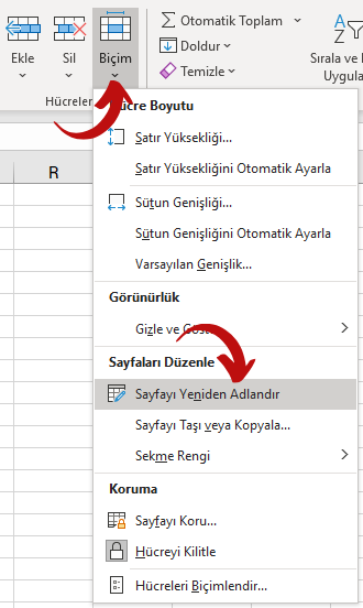
2- Right-click the Sheet Tab

This method works in all versions of Windows, Mac, 365 and online Excel.

  1. Right-click the sheet tab of the worksheet you want to rename to open the context menu.
  2. Click Rename on the menu list to emphasize the current sheet name.
  3. Type a new name for the worksheet.
  4. Press Enter to complete renaming the worksheet.
  5. The new name should be displayed on the sheet tab.


3- Access the Ribbon Options with your mouse

çalışma sayfalarını adlandırma

This method works in all versions of Windows, Mac, 365 and online Excel.

  1. Click the sheet tab of the worksheet to be renamed to make it the active page.
  2. Click the Home tab of the ribbon.
  3. Click Format on the Cells to open the drop-down menu.
  4. Click Rename Sheet to emphasize the sheet tab on bottom of the screen.
  5. Type a new name for the worksheet.
  6. Press Enter to complete renaming the worksheet.


Things to pay attention to while naming a worksheet:

  • Page name cannot be blank.
  • It cannot consist of more than 31 characters.
  • It cannot contain any of these characters: / ? * : [ ] For example, 05/04/2020 cannot be a valid worksheet name but 05-04-2020 can be.
  • It cannot start or end with an apostrophe (‘), but it can be used between texts and numbers in the name.
  • It cannot be named “History“. This is a special dictionary used for special purposes within Excel.


You can click here to get more information.

See you in other posts, bye. 🙋🏻‍♂️
You can share this post with your friends and enable them to get informed as well. 👍🏻

Create Custom Rules in Conditional Formatting

I will be talking a bit about how you can create custom rules for conditional formatting. Of course, to be able to create these rules, you need to be able to write formulas, at least a bit. I will tell you about how to create simple formulas and use them in conditional formatting. As you get better at writing formulas, I am sure that you will create better rules. You can take a look at our blog to find other articles about the other features.


WHAT IS CONDITIONAL FORMATTING?

 koşullu biçimlendirme

One of the most frequently used features in Excel is Conditional Formatting. This feature is usually used to color and highlight backgrounds of certain cells that comply with a specific rule. It is found within Styles in the Home menu. There are some available rules you can use. When the available rules are not enough for you, you can create your own rules and format the cell in compliance with those rules. Of course, for this you need to know how to write formulas like I have mentioned above.

We can see the available prepared rules when we choose Conditional Formatting like you can see below. We can easily format by color, text, and date. If the available rules are not enough for you, then you can choose “Use a formula to determine which cells to format” from the New Rule option and highlight the cells that comply with your rules by writing to the formula into the related field. If we want, we can create more than one Conditional Formatting in a field. We can use the Manage Rules option to see and change the conditions of these formats.

You can use the Clear Rules option to clear rules in a part of the page or in the whole page.

Let’s dig a bit deeper with practical examples.

APPLY CUSTOM RULES IN CONDITIONAL FORMATTING

HIGHLIGHT TEXTS

In our first example, we will make a simple application about creating custom rules in conditional formatting. Let’s detect and highlight backgrounds of texts in the field we determine. For this, we need a function that would detect if a value in a cell is text or not. This function is called: ISTEXT. We will be able to automatically highlight the data if they are text in the specified field.

You can see how to do it in this GIF and do the same thing for your work.

emetinse ile koşullu biçimlendirmede metin olanları renklendirmek


HIGHLIGHT WEEKENDS

Let’s detect the weekends of the dates in a columns and highlight their backgrounds for our second example. We will need a function for this as well, and it is called WEEKDAY.  With this function, we can find out which day a date is in its week. I.e, it will give us a number between 1 and 7; and we will highlight the dates that happen to be weekends by writing a rule of if the number is bigger than 5.

First, I want to do a live application of this formula for you to do it live as well and comprehend it better. After writing the formula to the cell, we will copy that formula and paste it to the use formula section in conditional formatting.


koşullu biçimlendirmede hafta sonunu renkli göstermek


And as the last step, we will write this formula to the related field, click on format and complete the action.


koşullu biçimi uygulama


If you say that you need more information, you can check Office Support.


See you in other articles, bye. 🙋🏻‍♂️
You can share this post with your friends and enable them to get informed as well.👍🏻

Get a Picture from a Cell with a Formula

In this article, I want to explain you how to get a picture to a cell with a formula. As you know, we can get the data of the columns we want from a table by looking up for a value on the specified table with lookup and reference functions like VLOOKUP but we can only get the data inside a cell. At this point, what we want to tell you is that if there is a picture in the are we want to get, we can get it with a formula. By the way, we would like you to read and analyze our articles about Office, you can find them on our blog.


Get a Picture to the Cell with a Formula

Let’s say that we have two different pages. On one page, there are products, brand names etc. and on the other page there are product and brand pictures. We can get the picture on the second page next to the product and brand name on the first page with a formula that we’ll write. While doing that, as you’ll see below, we need to define names. We cannot get the picture in a cell without defining names.


Here is how you do it step by step:

  • Create a Data Verification list with brands.
  • Write the main formula necessary for this action.
  • Name the formula we created with the Name Manager.
  • Complete the process by assigning the name to the picture.


Let’s start understanding how to do it with pictures! 😀

We talked about creating a data verification list first, let’s take a look at it.

veri doğrulama listesine almak


We took the brand names to the data verification list.Let’s write the formulas that will do the job. I am leaving the formula here, you can see how I write it in the gif below.

=İNDİS('6-1'!$B$2:$B$6;KAÇINCI('6'!$A$2;'6-1'!$A$2:$A$6;0))


formülle resim getirme formülü


Now we’ll name the formula I have written, assign the picture on the first page and complete this action.


formüle ad verme


As you can see, we have learned how to get a picture to a cell with a few steps.. We have called a picture on another page to the active page with brand names. You can execute this kind of examples by getting pictures dynamically.

Also, you can get more information about defining names on Microsoft Support.


See you in other articles, bye.🙋🏻‍♂️
You can share this post with your friends and help them get informed. 👍🏻