

I will be talking a bit about how you can create custom rules for conditional formatting. Of course, to be able to create these rules, you need to be able to write formulas, at least a bit. I will tell you about how to create simple formulas and use them in conditional formatting. As you get better at writing formulas, I am sure that you will create better rules. You can take a look at our blog to find other articles about the other features.
WHAT IS CONDITIONAL FORMATTING?
One of the most frequently used features in Excel is Conditional Formatting. This feature is usually used to color and highlight backgrounds of certain cells that comply with a specific rule. It is found within Styles in the Home menu. There are some available rules you can use. When the available rules are not enough for you, you can create your own rules and format the cell in compliance with those rules. Of course, for this you need to know how to write formulas like I have mentioned above.
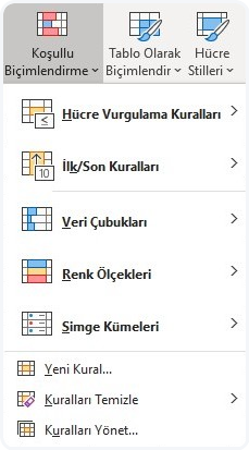
We can see the available prepared rules when we choose Conditional Formatting like you can see below. We can easily format by color, text, and date. If the available rules are not enough for you, then you can choose “Use a formula to determine which cells to format” from the New Rule option and highlight the cells that comply with your rules by writing to the formula into the related field. If we want, we can create more than one Conditional Formatting in a field. We can use the Manage Rules option to see and change the conditions of these formats.
You can use the Clear Rules option to clear rules in a part of the page or in the whole page.
Let’s dig a bit deeper with practical examples.
APPLY CUSTOM RULES IN CONDITIONAL FORMATTING
HIGHLIGHT TEXTS
In our first example, we will make a simple application about creating custom rules in conditional formatting. Let’s detect and highlight backgrounds of texts in the field we determine. For this, we need a function that would detect if a value in a cell is text or not. This function is called: ISTEXT. We will be able to automatically highlight the data if they are text in the specified field.
You can see how to do it in this GIF and do the same thing for your work.
HIGHLIGHT WEEKENDS
Let’s detect the weekends of the dates in a columns and highlight their backgrounds for our second example. We will need a function for this as well, and it is called WEEKDAY. With this function, we can find out which day a date is in its week. I.e, it will give us a number between 1 and 7; and we will highlight the dates that happen to be weekends by writing a rule of if the number is bigger than 5.
First, I want to do a live application of this formula for you to do it live as well and comprehend it better. After writing the formula to the cell, we will copy that formula and paste it to the use formula section in conditional formatting.
And as the last step, we will write this formula to the related field, click on format and complete the action.
If you say that you need more information, you can check Office Support.
See you in other articles, bye. 🙋🏻♂️
You can share this post with your friends and enable them to get informed as well.👍🏻