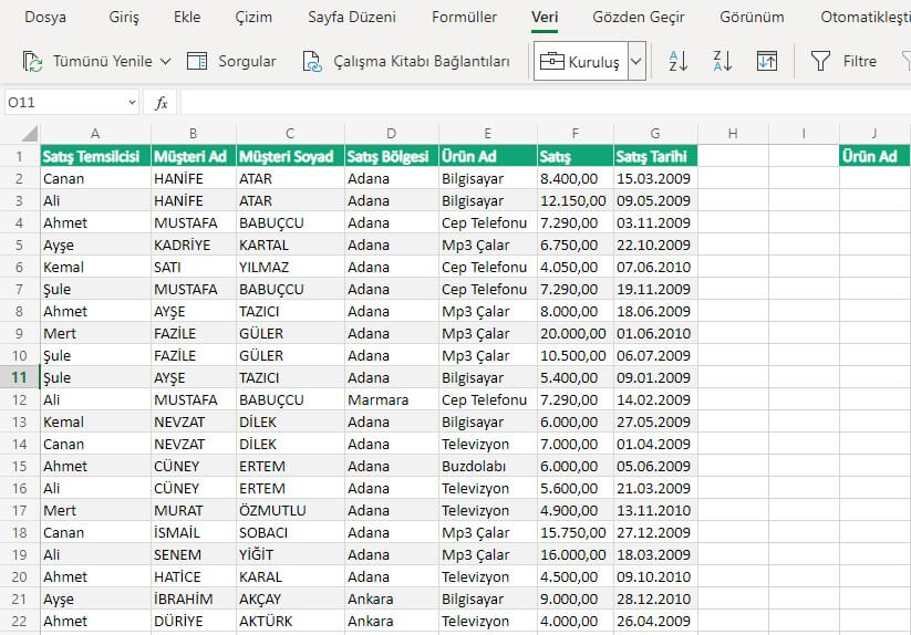
In this article, we will be talking about the benefits of the table format of the data range in Excel. When we write titles and enter data under those title or when working on a prepared file we received, we say that we have prepared a table. But the data range we call a table is not a table for Excel yet. For it to be seen as a table, you need to format the data range as a table. At that point, it allows us to use a lot of features that table format allows us.
Now let’s take a look what we need to do before creating to table to use some features and how we do them after formatting as table. By the way, it would be very helpful to write the articles on our Blog when you have a chance. If you wish, you can read a detailed article on Office Support.
Choose Style for the Table Format
We can use this feature by choosing Format as Table in the Styles group in Home tab. Choose any cell on your data and click the Format as Table command and choose the table style you want. You will have turned your data into a table quickly. Don’t forget: Everything added to the page later is an object. An image, shape, chart, table, slicer etc. all of them are objects and a menu with features of objects added later is added to the Ribbon.
You can apply this feature easily with the shortcut keys.
Choose any cell on your data and turn your data into a table with the
- CTRL + T
shortcut.
Now, let’s see what kind of features our data range gained with such a simple shortcut.
Benefits of the Table Format
- When you choose a cell on the table and move upwards and downwards, the column titles will be the titles of your table. Thus, you don’t need to use the Freeze Top Row feature in the Freeze Panes field in the View tab.
- A style is applied to our table automatically and each row is colored as dark and light successively one-by-one. And this creates a nice image.
- When you keep entering data under the table or next to the table, your table gets longer and wider. And this enables the data we enter later to be included in the table and everything to be accepted as a whole.

- Before applying the table format, when we want to get the 18% VAT in the Sum field written to the next column; we had to write the formula into a cell and drag it down first. If there are blank rows in between, we had do drag down again. But, when we format it as a table, it is enough to write the formula and press Enter for the formula to be applied on the whole column.
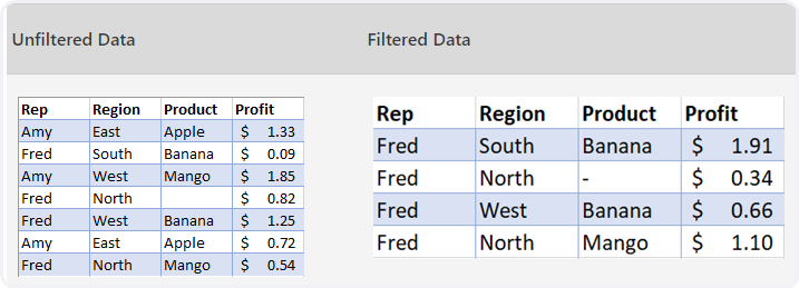
- When we turn the data into a table, a menu named Table Design or just Design is created in the Ribbon. This menu contains the features that we can use for our table. One of the most important features is the Slicer feature that we are familiar with from the Pivot Table. This feature enables us to filter the area we want on our table with one click.
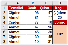
- It allows us to add functions like sum, average, count, min, max easily when we filter on the table. You can take a look at the other Table Style Options.
- When you create a Pivot Table from the data range, you have to choose Change Data Source most of the time when new data is added outside the field specified as the range. Considering that you add new data to your table every day, you will have to choose Change Data Source and specify the new data range all the time. But, when we turn our data into a table, the data we add under it or next to it will be accepted as a part of the table and is within the data range. Thus, it will be enough to Renew for the data to be reflected on the Pivot Table.
- In the formulas, we get to specify the data range by writing the table’s name without having to choose the whole table.
We have seen a lot of positive features till now and we obtained them with CTRL + T only.
Big or small, we recommend you to use Format as Table while working with data.
This way, you will be able to use the features above that will make you gain visualization and speed.
Convert to Range
Lastly, when you want to convert your table to data range again, you have two options.
- By choosing Convert to Range in the Table Design or Design menu.
- By right-clicking a cell on the table and choosing Convert to Range from Table.
I hope that this was a helpful article for you.
You can share this article with your friends and help a lot of people get informed as well.
Good bye. 👍🏻


 feature of Excel.