The RANDARRAY Function

In this article, I will be talking about one of the new dynamic array functions: the RANDARRAY function. Sometimes we need a data table filled out with random data. With this function, you can quickly fill as many rows and columns with numeral data. And you can find our articles about other functions on our blog.

WHAT DOES IT DO

The RANDARRAY function returns an array of random numbers. You can specify the number of rows and columns to fill, minimum and maximum values, and whether to return whole numbers or decimal values. The function returns a random set of values between 0 and 1 if you don’t enter an argument. For example, you can create a 20-row and 5-column table that contains whole numbers between 50 and 500 quickly in a few seconds.You will see an example below.

SYNTAX

=RANDARRAY([rows],[columns],[min],[max],[whole_number])This function has 5 arguments.
All of them are optional.

Now, let’s take a look at these arguments and what they mean, and what we will give them.

[rows]

Optional

The number of rows to be returned
[columns]

Optional

The number of columns to be returned
[min]

Optional

The minimum number you would like returned
[max]

Optional

The maximum number you would like returned
[whole_number]

Optional

Return a whole number or a decimal value

  • TRUE for a whole number
  • FALSE for a decimal number.


WORKING CONDITIONS

  • If you don’t input a row or column argument, RANDARRAY will return a single value between 0 and 1.

  • If you don’t input a minimum or maximum value argument, RANDARRAY will default to 0 and 1 respectively.
  • The minimum number argument must be less than the maximum number, otherwise RANDARRAY will return a #VALUE! error.

  • If you don’t input a whole_number argument, RANDARRY will default to FALSE, or decimal value.
  • The RANDARRAY function will return an array, which will spill if it’s the final result of a formula. This means that Excel will dynamically create the appropriate sized array range when you press ENTER. If your supporting data is in an Excel table, then the array will automatically resize as you add or remove data from your array range if you’re using structured references. For more details, see this article on spilled array behavior.

  • RANDARRAY is different from the RANDfunction in that RAND does not return an array, so RAND would need to be copied to the entire range.
  • An array can be thought of as a row of values, a column of values, or a combination of rows and columns of values. In the example above, the array for our RANDARRAY formula is range D2:F6,or 5 rows by 3 columns.
  • Excel has limited support for dynamic arrays between workbooks, and this scenario is only supported when both workbooks are open. If you close the source workbook, any linked dynamic array formulas will return a #REF! error when they are refreshed.


USE OF THE FUNCTION

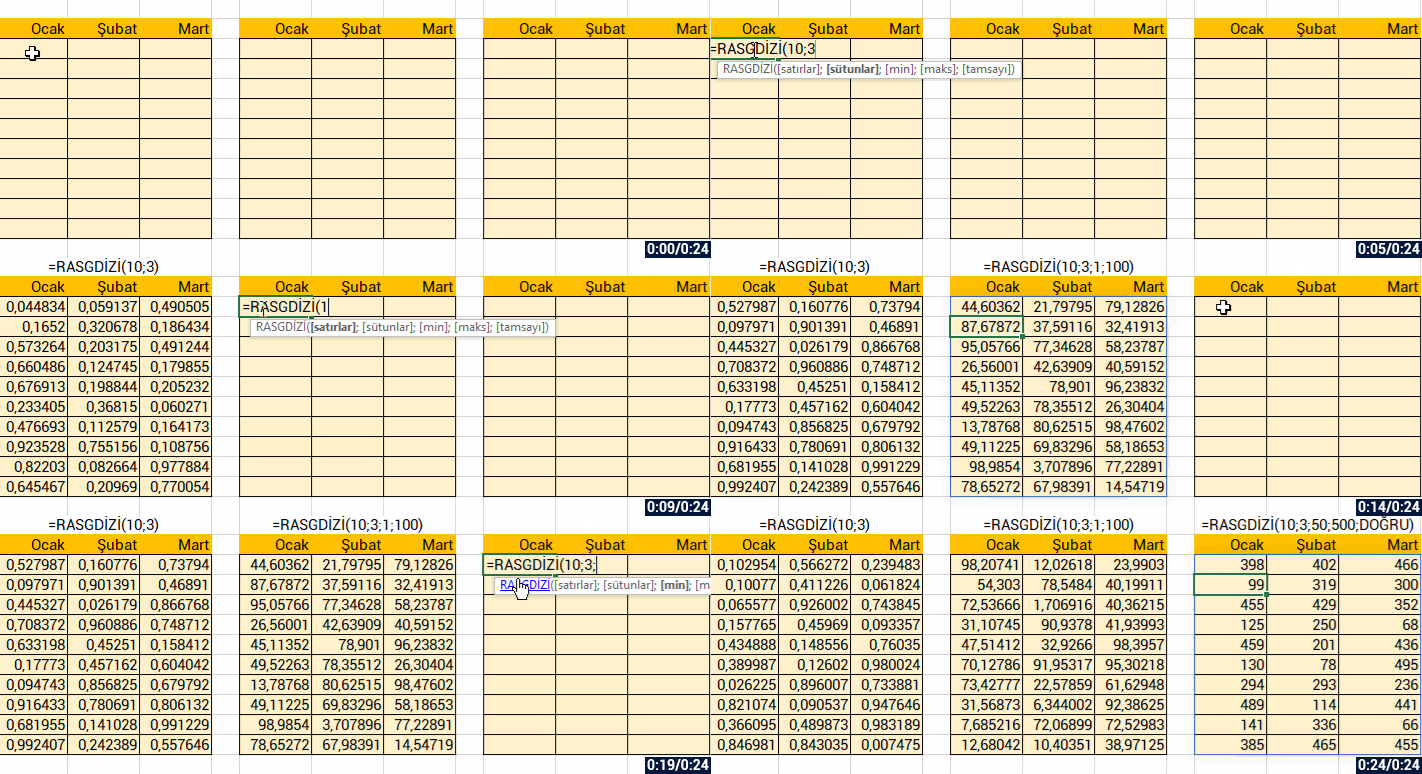
Now, let’s see how this function works with 3 different examples. First, we will determine rows and columns. And then we will give row, column, min and max number values and return a retrospective array. And then, we will request the numbers to be returned to be whole number. The image we will obtain is going be like this:


excel rasgdizi farklı örnekler


See you in other articles, bye. 🙋🏻‍♂️
You can share this post with your friends and get them informed as well. 👍🏻


Office Insider – What Happened in March?

NEW FEATURES/FIXES


You can find and follow all monthly Office insider new features and fixes (updates) on our blog. 👍🏻  Officer insider gets updates and new features regularly. It is important to follow these Office insider updates and use them in terms of increasing your knowledge. Now let’s take a look at what kind of changes happened in Office insider in the month of March.


March 28, 2020

outlook iconOutlook

Calendar visual refresh

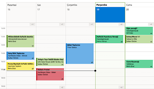
Last year, we brought you a refreshed mail experience, and, this year, it is the calendar’s turn to get a facelift! The updates are fresh but familiar so, as a seasoned Outlook user, you can jump in and be more productive right away.

Learn more.

Takvimde çalışma haftasının resmi.

Notable Fixes

  • This change addresses delays when processing images with malformed or invalid protocol information.
  • This change fixes an issue where the latest changes to draft emails were not being updated.
  • Fixed an issue where right-mouse clicking on a file and using ‘Send to’ would not work.
  • Fixed an issue where if a user had a customized the search path for the Address book, Outlook’s name resolution scope would be limited to the customized path rather than including the Global Address List (GAL).
  • Fixed an issue where within a set of returned search results, sorting the results by Categories would not display the Category colors.


PowerPoint iconPowerPoint

Synchronize changes while you are presenting

For years, PowerPoint didn’t allow changes made to slides by others to be displayed while presenting. This ensured that the presenter was in full control of the content being shared. No one could revise slides, either accidentally or maliciously. It also ensured that all of your computer resources were used for slideshow rendering. A concern that is especially important if you are running on a low-end machine.

However, while some presenters may still desire this original design, we’ve heard from others that they are seeking more flexibility. With an increased focus on collaboration and real-time updates, we’re excited to make available the ability to synchronize changes whenever they are made, even when the presentation is in Slide Show mode.


How it works

You can synchronize changes in two ways: automatically or manually.

Automatically update slide content

1. Select the Keep Slide Updated check box on the Slide Show tab on the ribbon.

PowerPoint

2. Start the presentation by selecting the appropriate button on the Slide Show tab.


Synchronize changes


3. Whenever an update to a slide is made and detected, the content is automatically updated and visible in the slide show being presented.

Manually update slide content

1. Clear the Keep Slide Updated check box on the Slide Show tab on the ribbon.

Synchronize changes


2. Start the presentation by selecting the appropriate button on the Slide Show tab.

3. Whenever an update to a slide is made and detected, an Update Slides button appears at the top of Presenter View.


Synchronize changes


4. Click the Update Slides button to manually synchronize the slide content.

word new iconWord

Notable Fixes

  • Fixed an issue where the functionality to post comments was disabled.
  • This change addresses delays when processing images with malformed or invalid protocol information.
  • This change addresses an issue where the account manager would not dispatch messages resulting in a hang with third party applications.
  • This change fixes an issue where the Table of Contents would get updated with heading styles which were not present in the document.
  • Fixed an issue where digital signatures saved in Word documents would be removed when mailing the documents.


excel new iconExcel

Notable Fixes

  • This change addresses delays when processing images with malformed or invalid protocol information.


msproject new iconProject

Notable fixes

  • Fixed an issue where the ‘ProjectBeforeTaskChange’ Visual Basic Applications (VBA) event did not fire when a user clicked the “Inactivate” button found on the Tasks Ribbon within the Scheduling grouping.
  • If you set predecessor or successor details from within a Form type view, the ProjectBeforeTaskChange Visual Basic Applications (VBA) event didn’t always capture the changes. For example, if you deleted a dependency and clicked OK on the form, the event did not fire. This behavior has been fixed.
  • Fixed an issue where the latest values for the Actual Cost of Work Performed (ACWP) would not be displayed after making a change, such as a date change.
  • Fixed an issue where opening a project using the Most Recently Used (MRU) menu opened the project file with Read/Write access.
  • This change fixes an issue where if you created a manual task with a start date and a time (but no duration), it would be displayed with an incorrect time on the timeline.
  • Fixed an issue where printing a timeline using Hijri calendar would result in a month being skipped or duplicated in the print view.
  • This change addresses an issue where working in Team Planner with GDI objects, could result in the over allocation of GDI objects and create low memory conditions.


March 13, 2020  

word new iconWord, excel new iconExcel,PowerPoint new iconPowerPoint andoutlook new iconOutlook

Sensitivity labels

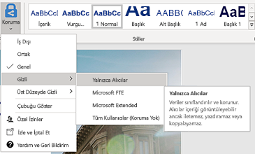
You can now apply a sensitivity label that your organization has configured to prompt you for custom permissions. Learn more

How to Access

If your organization has set up Sensitivity tags in Microsoft Information Protection and enabled users to assign permissions, you can access them. For example, choose Home> Protect, then select the label you want to apply to the document, workbook, presentation, or email.

İzinlere nasıl erişileceğini gösteren Word belgesinin resmi.

outlook new iconOutlook

Notable Fixes

  • Addresses an issue that caused the “Last Modified”; date on a file to be updated when adding an attachment to a mail or saving an attachment from a mail by dragging and dropping it (as opposed to via a menu).
  • Addresses an issue that caused hitting enter in the expanded find pane to fail to start a search, requiring instead that users click on the search button.
  • Fixed an issue where search shows no information about users when the option to “Show user photographs when available” is disabled.


word new iconWord

Notable Fixes

  • Fixed an issue when typing or editing a comment and using Ctrl+A would result in selecting text in the canvas instead of selecting text just within the comment card.
  • We fixed an issue in which the alignment of words in a document gets scrambled when tried to edit after printing using Quick Print.
  • We fixed an issue when merging two documents into one document.
  • Fixed an issue where marking revisions involving equations could result in a failure when saving the file.


excel new iconExcel

Notable Fixes

  • Fixed a performance issue that users may have experienced when programmatically editing a large range of cells.
  • Fixed a performance issue that occurred when opening csv files with Japanese environments.


msproject new iconProject

Notable Fixes

  • Fixed an issue where summary task dates weren’t always getting calculated correctly.
  • Fixed an issue where the OnUndoOrRedo event doesn’t fire without first running the OpenUndoTransaction method.


access new iconAccess

Notable Fixes

  • Fixed an issue where international versions of Access were displaying English strings in the user interface.


PowerPoint

New Features

Look above.


March 10, 2020

excel new iconExcel,word new iconWord,PowerPoint andoutlook new iconOutlook

Pick the perfect color

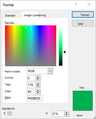
We heard you! Converting Hex colors to RGB values is now a thing of the past. For any property where you can define a color, click the appropriate button in the ribbon (such as the Font Color button) and click More Colors. Then, in the Colors dialog box, click the Custom tab and enter the Hex color value in the Hex box, for example, #0F4C81 or 444.

Learn more

Onaltılık bilgiler alanını gösteren renkli kutu.

excel new iconExcel

Automatically use new data types*

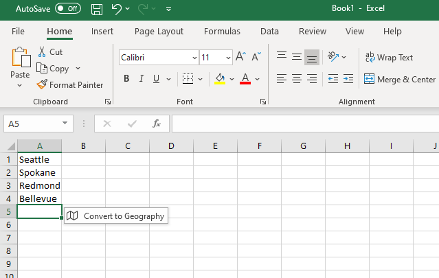
When you type a data value that resembles a possible stock or geographic location, Excel offers to convert it to the appropriate connected data type – Stocks or Geography. Give it a try!

Type in several geographic locations (such as “Seattle”, “London”, or “Tel Aviv”) or stock ticker symbols (such as “MSFT”, “ADBE”, or “AAPL”) in separate cells in a column.

When Convert to Geography or Convert to Stocks appears to the right of the selected cell, click on it.

Verileri dönüştür kutusunun bulunduğu Excel çalışma kitabı.

* This feature is only available in English right now.

outlook new iconOutlook

Drag emails to a group you own

As a group owner, you can now move and copy messages and threads by dragging and dropping them from your mailbox to the groups’ mailbox. Once moved, the content is visible to all the group members, and anyone can read the messages and participate in the conversation.

Learn more

Better search results, faster

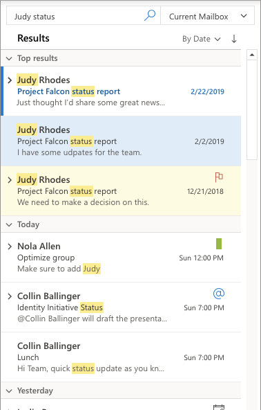
The Search experience in Outlook just got a facelift! It is now more reliable, intelligent, and faster than ever. Also, any search entry is now being spell checked and, if errors are detected, helpful suggestions are offered to ensure that you get to the results you’re looking for. Finally, notice that the most relevant search results are presented at the top of the results list, making access faster.

Arama öğelerinin vurgulandığı Outlook posta kutusu resmi.

PowerPoint

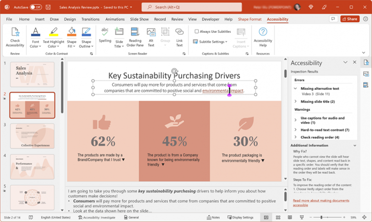
Diagrams get connector support

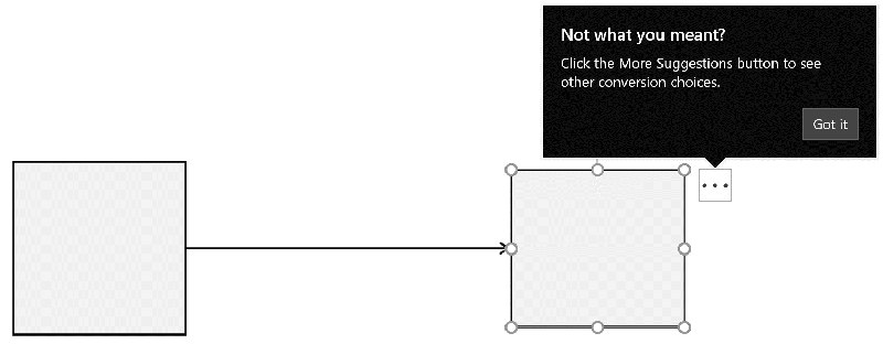
Now, the converted lines between objects are connectors anchored to the shapes.

Ink conversion is also easier than ever with just clicking the Convert your ink button Convert your ink button. Select the converted object again to be able to access other conversion alternates, to make sure the conversion fits your needs. Give it a try! Give it a try!

Sağda siyah bağlayıcı dönüştürme kutusuyla boş beyaz kutular.


March 6, 2020  

outlook new iconOutlook

Notable fixes 
  • We fixed an issue that was preventing users from attaching a file to their mail messages when that file was open in another application.
  • We fixed an issue where creating a rule with Outlook Web Access did not persist to the Exchange server and resulted in a conflict.
  • We fixed an issue with Outlook that wouldn’t show the drop-down list in the “From” field when using dark mode.


word new iconWord

Notable fixes 
  • We fixed an issue that made the User Principal Name (UPN) people case-sensitive, e.g., [email protected] would fail to match [email protected], and prevented users from accessing the SharePoint Sites service.
  • We fixed an issue that prevented the Compare feature from working when the document was protected for editing.


PowerPoint

Notable fixes 
  • We fixed an issue that made the User Principal Name (UPN) people case-sensitive, e.g., [email protected] would fail to match [email protected], and prevented users from accessing the SharePoint Sites service.
  • We fixed an issue where the recommended thumbnails flashed when hovering your mouse over the thumbnails. In some cases, this could cause PowerPoint to crash.


excel new iconExcel

Notable fixes 
  • We fixed an issue that made the User Principal Name (UPN) people case-sensitive, e.g., [email protected] would fail to match [email protected], and prevented users from accessing the SharePoint Sites service.


We compiled all the new features and fixes in March in Office insider. Hope to see you in our other articles, bye bye. 🙋🏻‍♂️
You can share this article with your friends and family to help them get information about Office insider updates released in the month of March. 👍🏻 

Methods of Copying a Cell As a Picture

In this article, we will be talking about methods of Copying a cell as a picture in Excel. There are three methods we can use for this action. You will see these methods and our recommendations in our article. You can find a lot of features like this on our blog, don’t forget to follow.


WHY DO WE NEED THIS?

Sometimes we want to transfer the image of a range in our table as a picture to other office applications or any application. For example, when we want to copy the selected table range and directly paste on Outlook, Word etc. it will be pasted as a table. This way, it will be possible to be edited. So, it would be better to copy the cell as a picture or paste the copied data as a picture.


METHODS OF COPYING A CELL AS A PICTURE

Our first method

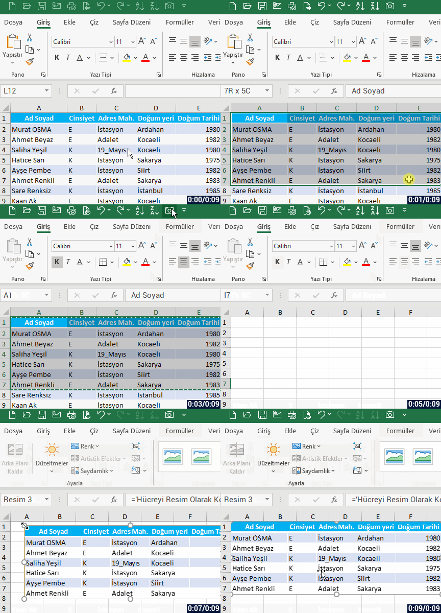
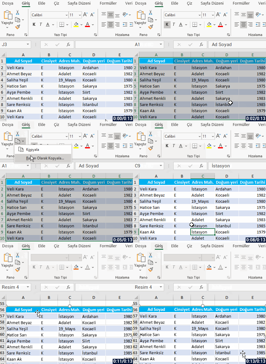
is through the Copy as Picture in the Clipboard on the Home tab.

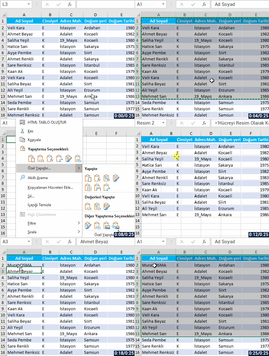
hücreyi resim olarak kopyalama


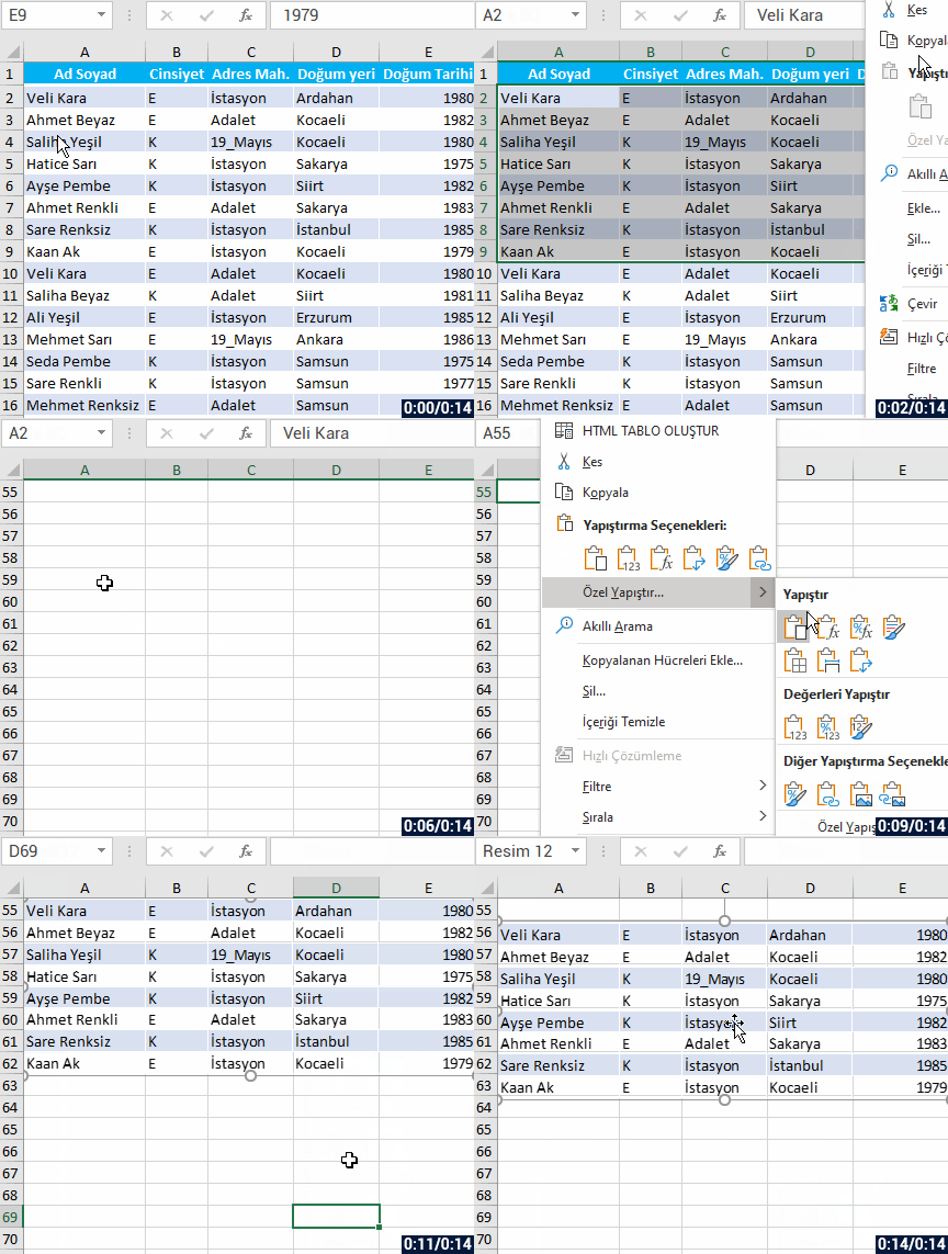
Our second method is choosing the Picture option in the Paste Special Option after selecting and copying the cell range.

özel yapıştırma seçeneği


This way, when you paste it as a picture, the data on the picture won’t change when the data in the cell you’ve copied changes. But when you paste as Linked Picture in the paste special options, you can see that the cell changes when you make a change in the cells you’ve copied. This will provide us with a dynamic look.

The same way, you can view the change you make in the cell range you’ve copied in Excel in other Office apps like Word and PowerPoint too by choosing the Paste as Linked Picture option from the paste special options.


Now let’s give an example of paste as a Linked Picture. You will see that when we change a data in the copied table, the change will go through in the picture as well.


bağlı resim


Our third method is to take a picture of the cell range we want with the Camera feature in Excel and then transmit it from the memory to the cell we want to paste the picture into. For this, you can add the Camera feature to the Quick Access Toolbar with these steps:

  • File
  • Options
  • Quick Access Toolbar
  • Commands Not in the Ribbon
  • Camera
  • Add
  • OK

After executing these actions, you will see the Camera Iconhücreyi resim olarak kaydetme kamera özelliği  on the Quick Access Toolbar. I recommend you to have the camera feature there all the time.

Now, let’s see how easy it is to copy and paste the cell as a picture with this feature.

hücreye resim eklemek


You can save the cell range as a picture with these methods we’ve shared with you. If you want, you can get extra information on Microsoft Support.


See you in other articles, bye. 🙋🏻‍♂️
You can share this post with your friends and help them get informed as well.👍🏻

The SEQUENCE Function

In this article I will be talking about the SEQUENCE Function that is one of the dynamic array functions. It allows us to create a list of sequential numbers in an array when we want to give a sequence number in a column or we give a starting number and indicate the increase value. We can easily use it when we need to quickly create a data set. You can find articles about other functions on our blog.


WHAT DOES IT DO

The SEQUENCE Function -like I mentioned above- is a function similar to the Flash Fill option in the Fill field in Excel. For example, when we want to give a sequence number from 1 to 20, it is going to be enough for us to write =SEQUENCE(20). Or let’s say that you are going to create a 10-row and 5-column numeral data table. When we want these numbers to start from a certain number and increase by the value we indicate and fill the sequence like that, we can use this function. We can do extra special actions with the numeric values this functions returns us.


SYNTAX

=SEQUENCE(rows,[columns],[start],[step])

This function has 4 arguments.
The first one of these arguments is required and the other 3 are optional.

Now let’s take a look at what these arguments mean, i.e. what this function wants from us and what we will give it.

sıralı fonksiyon argümanları listesi


WORKING CONDITIONS

  • Any missing optional arguments will default to 1.
  • An array can be thought of as a row of values, a column of values, or a combination of rows and columns of values. In the example above, the array for our SEQUENCE formula is range C1:G4.

  • The SEQUENCE function will return an array, which will spill if it’s the final result of a formula. This means that Excel will dynamically create the appropriate sized array range when you press ENTER. If your supporting data is in an Excel table, then the array will automatically resize as you add or remove data from your array range if you’re using structured references. For more details, see this article on spilled array behavior.
  • Excel has limited support for dynamic arrays between workbooks, and this scenario is only supported when both workbooks are open. If you close the source workbook, any linked dynamic array formulas will return a #REF! error when they are refreshed.


USE OF THE FUNCTION

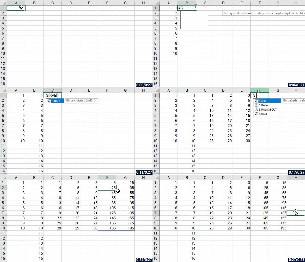
If you want, you can try to give a sequence number in a column. We can obtain a sequence of numbers starting from 1 for the specified number of rows and columns. If you wish, you can increase step by step by using the increment value. Let’s take a look at how to use the function.

sıralı fonksiyonu kullanımı


SPLIT THE DATA INTO COLUMNS EASILY

Now let’s have an example of the use in extra special actions…
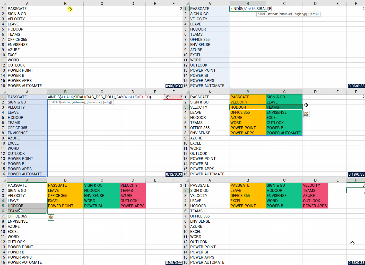
Let’s assume that there are dozens, hundreds, thousands of row of data in the A column, and you want to split that data into a few columns. Now, we can create the list easily with the numbers it returns with the logic of this function. In the example below, there are 16 rows of data in the A column. Let’s get these written equally in the A and B columns with a row gap.


sıralı function farklı kullanımı


See you in other articles, bye. 🙋🏻‍♂️
You can share this article with your friends and help them get informed. 👍🏻

coder by

LET : THE NEWEST FUNCTION

This week I will be talking about a function recently announced by Microsoft that only the Office Insider users can use: the LET Function. Like I mentioned in the FILTER function article, as the new dynamic string functions we will be able to execute a lot of actions more simply and quickly. And new features keep coming one after another. You can easily keep up-to-date by following our articles. 👍🏻


DEFINITION OF THE LET FUNCTION

In the announcement the definition goes like:

Have you ever had to repeat the same expression multiple times within a formula, created a mega formula or wished that you had a way to reuse portions of your formula for easier consumption? With the addition of the LET function, now you can!

The LET function assigns names to calculation results and makes it easier for you to reuse the parts of the formula. In a way, it means that we can Define Names in a function and use the name in calculation. Sometime when we are writing a formula, we need to state the same range or condition multiple time. the LET function will be helping as right at this point. We will name the value we have to use multiple times in a formula and we’ll indicate it with that name in the function.

The main benefits are:

1. Readability

No more having to remember what a specific range/cell reference referred to, what your calculation was doing or duplicating the same expression within a formula. With the ability to name expressions, you can give meaningful context to readers of your formula.

2. Performance

If you reuse the same expression multiple times in a formula, Excel calculates that expression multiple times. LET allows you to name the expression and refer to it using that name. Any named expression is calculated only once, even if it is referred to many times in the formula. This can significantly improve performance for computationally complex expressions.


SYNTAX

LET

(name1, value1, [name2…], [value2…], calculation)
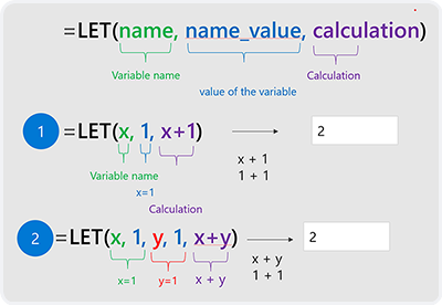
let fonksiyonu

This function consists of 3 basic arguments. Name and value arguments can be optionally increased.

The 3 basic arguments are required. For the function to work, there has to be indicated value and calculation arguments.

Let’s take a look at these arguments.

  • name1: The name for the 1st value
  • value1: The value to associate with the 1st name
  • name2 (optional): Additional names
  • value2 (optional): Additional values
  • calculation: The calculation to perform. This is always the final argument and it can refer to any of the defined names in the LET.


Deconstructing the parameters, there are two things to make note of

  1.  The names and their values must be in pairs. If there is a name but there is not a value, the function doesn’t work.
  2. The last parameter of the function is the calculation which can use the values you named. A properly structured LET will have an odd number of arguments.


ADDITIONAL REMARKS 

  • The last argument should be a calculation that returns a result.
  • Argument names are limited with the names that can be used in the Name Manager. For example, “a” is valid but “c” will not be a valid name since it coincides with the R1C1 reference styles.


This example will help you comprehend it better:

=LET(total; SUM(A1:A10); total * 3)

Let me give another example so that the software people can comprehend it better: in the formula below, I have created a variable called sum and gave it the 1 value. In the calculation part, I said add +2 to the sum variable and as a result, this function will return the result of 3.

=LET(SUM; 1; SUM+2)

If we want to take this a step further, I mean if we want to give double names and values, we can use it like this:

=LET(total, SUM(A1:A10), count, COUNT(A1:A10), total / count)

Here is another example:
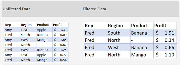
izinver fonksiyon örneği

Here, you need to FILTER the Fred in the first column with the new FILTER dynamic string and if there is a blank cell, you need to enter – (hyphen) icon.

Normally, we can solve this with a formula like this; if there is a blank cell in the result coming from the filter, write hyphen there, if there is no blank cells filter normally.

=IF(ISBLANK(FILTER(A2:D8;A2:A8="Fred"));"-";FILTER(A2:D8;A2:A8="Fred"))

But if you have noticed, we wrote this part twice in the formula; FILTER(A2:D8;A2:A8=”Fred”)

LET function says that you don’t need to write the same data twice.

=LET(filterCriteria, “Fred”, filteredRange, FILTER(A2:D8,A2:A8=filterCriteria),

IF(ISBLANK(filteredRange),”-“,filteredRange))


Let me give another example of this beautiful function and than end my article: 😊
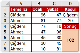
izinver fonksiyonu

The formula we need to write when we want to find the total data of February based on the conditions indicated above in D2 and D3 in the table above:

=IF(SUMIFS($C$2:$C$8;$A$2:$A$8;$D$2;$B$2:$B$8;">="&$D$3)<0;"Sum Incorrect";SUMIFS($C$2:$C$8;$A$2:$A$8;$D$2;$B$2:$B$8;">="&$D$3))

As you can see, we used SUMIFS two times in IF. We had to write it like that depending on our need.

But if we are to do it with the LET function, we only need to write the SUMIFS function once.

=LET(Sum;SUMIFS($C$2:$C$8;$A$2:$A$8;$D$2;$B$2:$B$8;">="&$D$3);IF(Sum<0;"Incorrect";Sum))


So much for the information I will share with you for now. If you want you can get more information here. As we start using this function in our daily lives, we will be sharing it with you. ⚡️


See you in other articles, bye. 🙋🏻‍♂️

You can share this post with your friends and help them get informed as well.👍🏻
The Weekday Function

In this article, I will be talking about on of the Date and Hour functions, the WEEKDAY Function that will helps us in our daily lives. This function returns the number that represents the day of the week of a specific date. It gives us a number between 1 and 7, and so we know which day of the week it is and do actions depending on that. If you want, you can get the details about the Weekday Function on support office. You can find our articles about the other function on our blog


WHAT DOES THE WEEKDAY FUNCTION DO?

The WEEKDAY Function

gives us a number stating the which day a date is in that week. For example, If we want to know which dates in a column are weekend, we can have them highlighted. Or, doesn’t matter which day the payment days are in the column, if your payment day is Friday you can organize all the dates on Friday in their weeks.

SYNTAX

WEEKDAY(serial_number,[return_type])

The WEEKDAY Function

has 2 arguments.
The first one of them is required and the other one is optional.

Now let’s take a look at the meaning of these arguments, i.e. what this function wants from us and what we will give it.

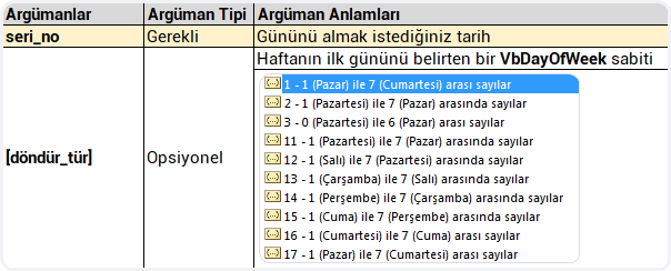
haftanıngünü fonksiyonu argüman listesi


WORKING CONDITIONS

The working conditions of the WEEKDAY function are:

  • Microsoft Excel stores dates as sequential serial numbers so they can be used in calculations. By default, January 1, 1900 is serial number 1, and January 1, 2008 is serial number 39448 because it is 39,448 days after January 1, 1900.
  • If serial_number is out of range for the current date base value, a #NUM! error is returned.

  • If return_type is out of the range specified in the table above, a #NUM! error is returned.

  • If the Calendar is Gregorian, the returned number represents the Gregorian day of the week.
    If the calendar is Hegira, the returned number represents the Hegira day of the week. If the calendar is Hegira Calendar,  the argument number is any number that can represent a date and/or time from 1/1/100 (Gregorian Aug 2, 718) to 4/3/9666 (Gregorian Dec 31, 9999).


USING THE WEEKDAY FUNCTION

In the Weekday Function, we choose the date that we want to get the day number for the Serial_number argument first. Then, we choose the type that we want the Return_type argument to return. We will come across the list where the first and last days of the week are stated. For us the option is the one with the number 2, where first day is Monday and the 7th day is Sunday. So, we choose the 2 option for the return_type argument and complete the formula.


 HIGHLIGHTING THE WEEKENDS

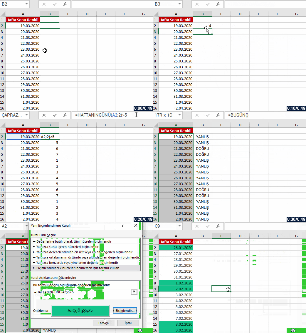
Let’s assume a list in which there are dates of March in a column. At the first glance, we cannot know which day those dates are. If you choose that column, choose Long Date as Format in the Number group in Home menu, you will get the day name and it might be useful for you. But we don’t want the day name, we want the weekends to be highlighted. We can achieve this with the WEEKDAY Function in the Conditional Formatting feature. Colors are very useful when it comes to analyzing a data.

Let’s start practicing with examples. You can apply these steps with me.
Unfortunately, an available rule that does what we want doesn’t exist in Conditional Formatting.
So, what do we do? We create our own rules with a formula, and achieve highlights based on that rule.
You can find and highlight the weekends like this.

weekday fonksiyon kullanımı


SETTING THE PAYMENT DAY AS FRIDAY

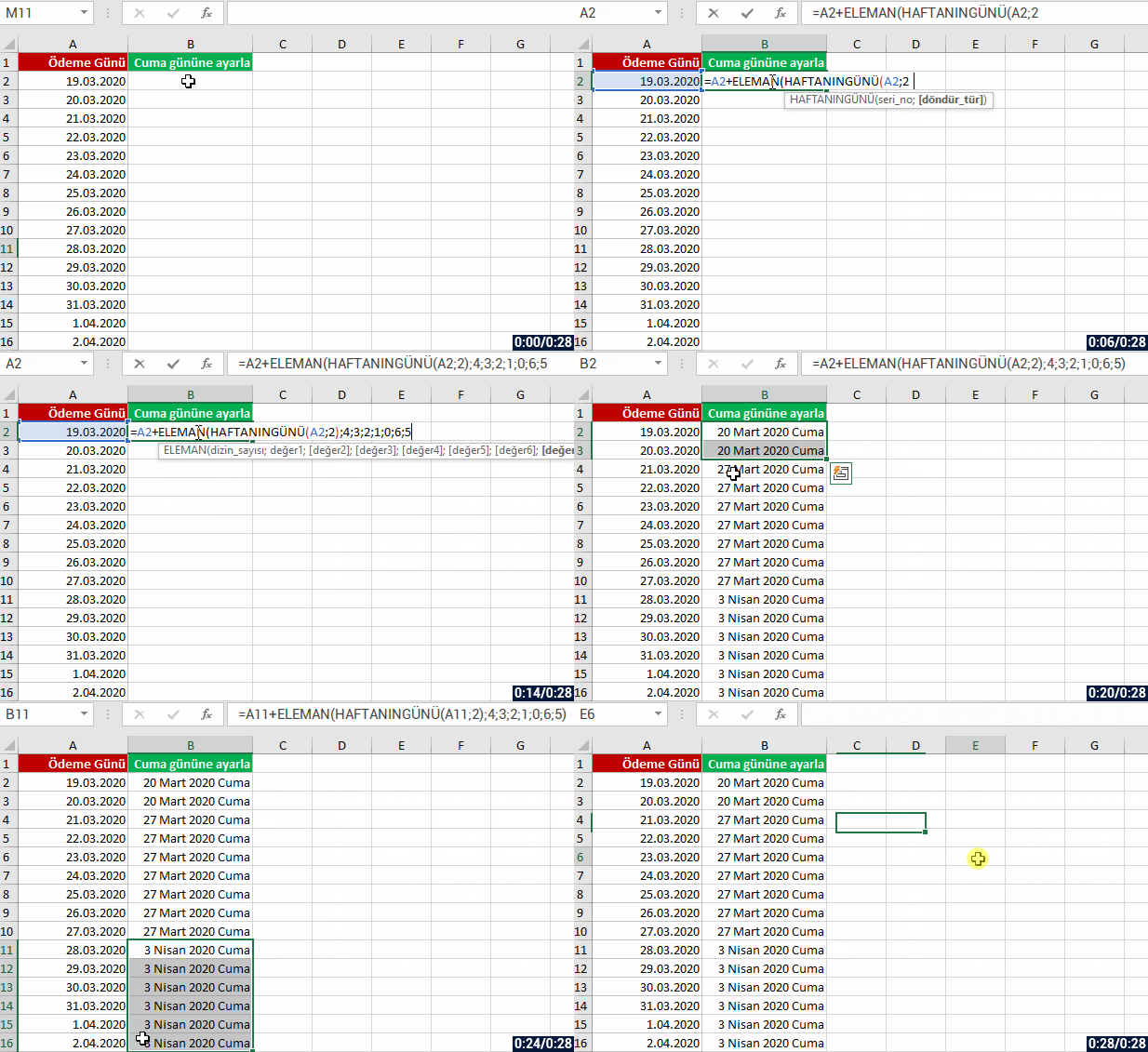
Let’s do an example of setting the payment day as Friday.
For this action, we will use the CHOOSE and WEEKDAY functions together.
Try to do this action as well and try to comprehend its logic by repeating few times.

weekday ile ödeme gününü cuma gününe ayarlama


See you in other articles, bye. 🙋🏻‍♂️
You can share this post with your friends and get them informed as well. 👍🏻

FIELDVALUE Function

In this article, we will be informing you about the FIELDVALUE Function used with the Linked Data Types. You can use the FIELDVALUE function to retrieve field data from linked data types like the Stocks or Geography data types.

bağlantılı veri türleri

There are easier methods for writing formulas that reference data types, so the FIELDVALUE function should be used mainly for creating conditional calculations based on linked data types.


SYNTAX

fieldvalue fonksiyonu söz dizimi

This function requires two arguments.
It is necessary to enter both of these arguments.

There are these independent variables in the syntax of the FIELDVALUE function:

  • value– Function returns all matching fields(s) from the linked data type specified in the value argument.
  • field_name– The name or names of the fields you would like to extract from the linked data type.

Description

  • The FIELDVALUE function returns all matching fields(s) from the linked data type specified in the value argument.

  • The FIELDVALUE function belongs to the Lookup & Reference family of functions.


Examples

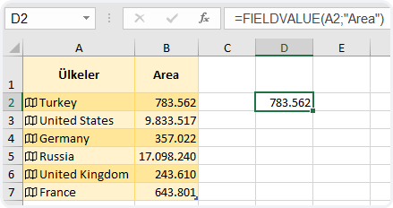
In the following basic example, the formula =FIELDVALUE(A2,”Area”) extracts the Area field from the geography data type for Turkey.

fieldvalue fonksiyonu örnek

Let’s list the data in the related field depending on the dynamic field choice about cities.

fieldvalue fonksiyonu örnek


Remarks

If you try to retrieve data from a non-existent data type field, the FIELDVALUE function will return the #FIELD! error. For instance, you might have entered “Field“, when the actual data type field is named “Area“. Double-check your formula to make sure you’re using a valid field name. If you want to display a list of field names for a record, select the cell for the record, and press Ctrl+Shift+F2 .

You can get more information on Microsoft Support.

See you in other articles, bye. 🙋🏻‍♂️
You can share this post with your friends and help them get informed as well.👍🏻
Office Insider Program – How to Join

What is the Windows Insider Program?

Microsoft Insider

was created for all Microsoft 365 users.

  • Office insider participants are granted first-hand access to new features and updates.
  • You can access dynamic array formulas.
  • In addition to this, you can share your comments about developments with the developers.

Click here to become an Office Insider member.


Access to the Insider Program

The procedure below is the simplest and most complete one.
For a long time it was blocked to go back to “standard” Excel version after you became an Insider .

But with this method you can change between channels anytime you want. smiley

When you go to File> Account menu and want to see information about Microsoft Account like synchronized files, you will see that there are 3 standard buttons that enable you to know your software version number and Office news. If you cannot see the Office Insider button there, follow the steps below.

1st Step: Add Office Insider Button to your Account

After yo do the settings below, you will see that the 4th button is added too. Click on the Insider button.
To do it you need to add a key into registry.  To open your registry type regedit on your Windows taskbar.

Normally Office, 16.0 and Common arrays are not on registry, you need to create them.

Path : HKEY_CURRENT_USERSoftwarePoliciesMicrosoftOffice16.0Common
Key Name: insiderslabbehavior
Value type : REG_DWORD
Value : 1

After you restart Office you will see that on the File > Account menu you have the Office Insider button.


2nd Step: Changing Office Channel 

Then, to see both of the recommended levels click on the Insider > Modification Level button.

You can see 2 levels of the available update by clicking on the popup menu: Monthly Channel or Insider.
Needless to say you need to accept terms of use to change the channel of your application.

3rd Step: Differences between the Two Programs


Insider Channel
This is the level that open the latest Office updates. Some of them didn’t have the chance to be tested by the developers or to be completed. Thus, it carries a risk to fail your Excel functions and collapse your workbooks (it is pretty common). However, it is the only way to access latest features like XLOOKUP.

My recommendation: Don’t set up this version on a professional environment. Would be better in a test machine.

Monthly Channel
This channel is not for test users, it is for very advanced level Excel users. This version opens up persistent features that are usually non-existent in Office standard version (six month channel). For example, to be able to use dynamic array functions you need to subscribe to one of the 2 levels of Insider. If not, you cannot use them.

For this, if some of your employees want to access features that require Insider, this channel is the one that needs to be set up.

4th Step: Update Office

Whatever Office level you choose, it is a must to update your Office.
Single selection of Office channel is not enough to open the Insider program.

After you choose one of the insider levels and click on update button, upgrade will start automatically.


5th Step: Restarting Excel

It is enough to restart your Office apps once or twice to see the changes.


Going back to the Six Month Channel (standard version)

The only thing you need to go back to the six month channel which is Office’s basic version:

  • Click on the Insider icon.
  • Uncheck Save to Preview new versions of Office option
  • Update Office again.


Don’t forget to check other articles on our blog.
You can share this article and make sure that many other people get informed as well.okay

Bye. 🙋🏻‍♂️

Office Insider – What Happened in June?


NEW FEATURES/FIXES


You can find and follow all monthly Office insider new features and fixes (updates) on our blog. 👍🏻  Officer insider gets updates and new features regularly. It is important to follow these Office insider updates and use them in terms of increasing your knowledge. Now let’s take a look at what kind of changes happened in Office insider in the month of June.


June 06, 2020


excel new iconExcel

Sheet View

Now you can sort and filter your Excel file while collaborating with others with Sheet View.
Thanks to this new feature, users working on the file together don’t get affected by the others’ sorting and filters.


Create PivotTables from Datasets in Power BI

Now, you can create PivotTables connected to datasets stored in Power BI in Excel with just a few clicks. This allows you to get the best of both PivotTables and Power BI.
Calculate, summarize, and analyze your data with PivotTables from your secure Power BI datasets.

Learn More

Notable fixes

  • An issue that caused the custom values in the chart axis not to be applied correctly has been fixed.
  • An issue that caused saving worksheets containing multiple formulas with defined names to take more time compared to now.

outlook new iconOutlook

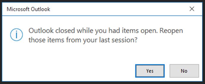
Quickly reopen items from previous session

We added an option to quickly reopen items from your previous session. Now you can automatically restore items that were open when Outlook got locked or closed.
To turn off the feature go to Options > General > Start up options.

önceki oturumdaki öğeleri yeniden açma

Notable Fixes

  • An issue where the Input Method Editor (IME) window would overlap the underlying text being entered via the IME when using multiple monitors with different resolutions has been fixed.
  • An issue where viewing a template when composing a new email message would result in a crash has been fixed.
  • An issue where users were unable to Exchange 2010 public folders after Outlook version 1911 has been fixed.
  • An issue where the Categorize button for group calendars in the Office Ribbon was disabled has been fixed.
  • An issue that caused users to experience a crash in Outlook when working with hyperlinks in plain text emails has been fixed.
  • An issue that caused Outlook to be unable to parse long file names encoded with RFC2231 has been fixed.
  • An issue that was causing Outlook users to experience intermittent hangs when using screen readers has been fixed.
  • An issue that resulted in the Online Archive dropdown in folder properties to be missing for users on high DPI monitors has been fixed.
  • An issue that would cause users with conflicting contacts to experience crashes in Outlook has been fixed.

word new iconWord

Notable fixes

  • An issue where timestamps in Comment panes were not based on the system locale time has been fixed.
  • An issue where comments between the web app and the desktop application were not in sync has been fixed.

PowerPoint

Notable Fixes

  • We fixed an issue where the slide editor from one slide would overlap on to the next slide.
  • We fixed an issue where a Comment pane that had been closed by the user would re-open automatically.
  • We fixed an issue where PowerPoint files with embedded charts/workbooks could result in failures when saving the file.
  • We fixed an issue with opening files from server-configured with Forms-based authentication.

msproject new iconProject

Notable Fixes

  • We fixed an issue that prevented orphaned tasks from being deleted or reassigned after the parent plan was deleted.


June 12, 2020

excel new iconExcel

Get Organization Data from Power BI using Data Types

Excel data types from Power BI are now rolling out to Insiders in organizations with Office 365 E5/A5 or Microsoft 365 E5/A5. Getting the information you need and easily refreshing it is critical to many everyday workflows.  You can access your company or organization information from Power BI as a data type in Excel, which expands your ability to bring in linked information in your spreadsheets.

Learn More 

Notable Fixes

  • An issue where the major gridlines of radar charts could not be formatted correctly has been fixed.

word new iconWord

Notable Fixes

  • An issue where the ability to clear formatting within the Comments pane via the Clear Formatting button in the Office Ribbon was not working has been fixed.
  • An issue where changing the size of a table when the ruler is not displayed caused other applications running in the background to start flashing has been fixed.
  • An issue where if Word had a list of more than 50 frequently opened documents, then after saving and opening a document, a revision history would be displayed even though no revisions were made to that document has been fixed.

msproject new iconProject

Notable Fixes

  • An issue where a baseline reset or update could change time-phased budget cost/work resources and the baseline could reflect incorrect budget values has been fixed.
  • An issue where the ProjectBeforeTaskChange event didn’t fire when there was a change to the project summary task, either the project start/task field has been fixed.

Access

Notable Fixes

  • An issue that caused Microsoft Access to fail to identify an Identity Column in a linked SQL Server table, which could cause rows to be reported as deleted incorrectly has been fixed.

June 19, 2020


excel new iconExcel

Notable Fixes

  • An issue where workbooks were read-only when the file only had read-only recommended has been fixed.
  • An issue where CustomUI XML for a custom ribbon tab was removed when saving to SharePoint /OneDrive has been fixed.

PowerPoint

Notable Fixes

  • An issue where a user’s presence color indicator was not getting refreshed in the co-authoring gallery during a live, co-authoring session has been fixed.

word new iconWord

Notable Fixes

  • An issue where the HTML hyperlink color was not being rendered correctly has been fixed.

outlook new iconOutlook

Notable Fixes

  • An issue where the Input Method Editor window would overlap the underlying text being entered via the IME when using multiple monitors with different resolutions has been fixed.
  • An issue where the dates in mini calendar failed to display in bold for users in Japan has been fixed.
  • An issue that prevented calendar reminders from showing exact times for the meetings coming up in less than a week has been fixed.
  • An issue that caused users to see the following error when closing an appointment that was previously saved has been fixed: “The item cannot be saved because it was changed by another user or in another window. Do you want to make a copy in the default folder for the item?”

msproject new iconProject

Notable Fixes

  • An issue where if Fixed Duration tasks are%100 complete but Actual Finish is not specified, the Task % Complete would display as less than 100% has been fixed.


Office Suite

Notable Fixes

  • An issue where the URLs that were not http or http based were not being displayed in the Most Recently Used list hast been fixed.


We compiled all the new features and fixes in June in Office insider. Hope to see you in our other articles, bye bye. 🙋🏻‍♂️
You can share this article with your friends and family to help them get information about Office insider updates released in the month of June. 👍🏻