Tag: office insider

EVERYTHING ABOUT THE VLOOKUP FORMULA

The VLOOKUP Function

Hello everybody,

As you can understand from the title, this article will be pretty long.
If you want to become an expert in the VLOOKUP formula, you can read this article till the end and apply it.

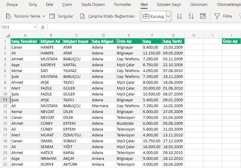
It is a function that everybody has heard of, everybody wants to learn and that everybody uses in Excel. We use the VLOOKUP function to find a value in the table.
Let’s explain it a bit: we use the VLOOKUP function when we search a data in a table or data range and want to get data from a column that corresponds to that data. For example: let’s assume that you have a personnel salary table. In one cell there is the personnel name, you can search your employee’s name and find out the salary they get easily.

SYNTAX

VLOOKUP (lookup_value, table_array, col_index_num, [range_lookup])

To express how the VLOOKUP function works simply:

=VLOOKUP (look for this; look in this table; if you find it bring me the one in the 2nd column; [TRUE – Approximate Match / FALSE – Exact Match])

Now let’s take a look at the arguments this function wants from us.

Argument name	Description
lookup_value (required)	The value you want to look up. The value you want to look up must be in the first column of the range of cells you specify in the *table_array* argument. For example, if *table-array* spans cells B2:D7, then your lookup_value must be in column B. *Lookup_value* can be a value or a reference to a cell.
table_array (required)	The range of cells in which the VLOOKUP will search for the *lookup_value* and the return value. You can use a named range or a table, and you can use names in the argument instead of cell references. The first column in the cell range must contain the *lookup_value*. The cell range also needs to include the return value you want to find. Learn how to select ranges in a worksheet.
col_index_num (required)	The column number (starting with 1 for the left-most column of *table_array*) that contains the return value.
range_lookup (optional)	A logical value that specifies whether you want VLOOKUP to find an approximate or an exact match: Approximate match – 1/TRUE assumes the first column in the table is sorted either numerically or alphabetically, and will then search for the closest value. This is the default method if you don’t specify one. For example, =VLOOKUP(90,A1:B100,2,TRUE). Exact match – 0/FALSE searches for the exact value in the first column. For example, =VLOOKUP(“Smith”,A1:B100,2,FALSE).

Working Conditions

When the required arguments are not entered, the function doesn’t work.
If the range_lookup optional argument is not entered, TRUE- Approximate match is considered as default.
The lookup_value always has to be on the far left (in first column) of the selected/indicated table array. But this situation can be overcome by writing different functions in VLOOKUP. (We will see this below.)
If the lookup_value is not found on the left of the table_array, #N/A error is returned.
If there is a multiple number of the data written into the lookup_value argument in the range indicated in the table_array argument, this function returns the record of the first data it found
it is not checked if the text written into the lookup_value argument is with uppercase or lowercase.
when a numeric data is written into the lookup_value argument, if the data type stated as table_array in the first column is text, #N/A error is returned. the same condition is valid in the opposite condition.
if a smaller number than 1 or a bigger number than the column number in the indicated table range or a text is written into the col_index_num argument, #VALUE! error is returned.
when a column is deleted from the field stated as table_array, #REF! error is returned.
1 and 0 can be written instead of TRUE and FALSE in the range_lookup argument.
If TRUE – Approximate Match is chosen, the table assumes that the first column will be sorted by number or alphabetically and looks for the most approximate value on the base. If you don’t specify a method, this method is used as default.
If FALSE- Exact Match is chose, if there is a value that is exactly the same with the data you have stated in the lookup-value argument is look for in the first column of the table_range.

THE BASIC USE OF THE VLOOKUP FUNCTION

You see a search sample suitable with the basic language and working conditions of the VLOOKUP function in the image below.

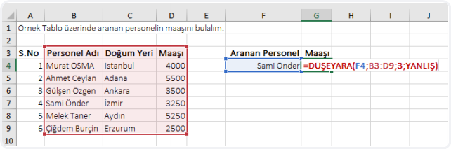
We have said that if you find the name Sami Önder in the B column which is the first column in the B3:D9 cell range , bring the data in the 3rd column of the selected range.

We have mentioned that we can write 0 instead of FALSE. With this FALSE expression, it i checked if there is an exact Sami Önder in the B column.

USING WILDCARD CHARACTERS

We can get the same result without having to write the full name we are looking for on the same table by using a wildcard character after writing the name only. Let’s brush up on the Wildcard Characters that we can use in Excel.

We have 3 different Wildcard characters.

Use	To find
? (question mark)	Any single character For example, sm?th finds “smith” and “smyth”
* (asterisk)	Any number of characters For example, *east finds “Northeast” and “Southeast”
~ (tilde) followed by ?, *, or ~	A question mark, asterisk, or tilde For example, fy06~? finds “fy06?”

The asterisk and question mark act as complementary character when it is in the beginning or end of a text in the lookup_value argument of the VLOOKUP function.
And ~ only limits the other wildcard characters by preceding them.

If the wildcard character precedes the text, it implies that the text ends with that. For example: *ali (if it ends with ali)
If the wildcard character is at the end of the text, it implies that the text starts with the. For example: ali* (If it starts with ali)
If the wildcard character is both in the beginning and at the end of the text, it implies that the texts contains that. For example: *ali* (if the text contains the word ali)
here is an example for the question mark: when you write ?ali, it means that there is a character (text, numbers or symbols) before the word ali.
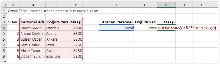
You can analyze this image as an example of the situation I have mentioned. ‘=F4&”*”

METHODS OF GETTING DATA FROM MULTIPLE COLUMNS

All Functions in Excel -except for the recently added dynamic array functions- return only one result.
When we get a result with the VLOOKUP formula, we might want to get the other data in the table by dragging the formula right.
Instead of writing the formula over and over again for each column, we can get data from the others column in the field we have stated as table_array when we drag the cell we have written the formula in right after adding a function to the col_index_num function that would change it as dynamic.
We can execute this action with a few methods. Now, let’s analyze these methods.

Our first method..

Let’s assume that we have a table like the one here.
We will get the data in the I.D. Number and Salary fields when we write the Name of the Personnel and drag it right.

We will have to write our formula correctly to execute an action like that.
And by correctly I mean using the cell styles correctly.
Which mean will we pin the cells while selecting the cell or cell range or not, or are we going to pin the row or column only?
As an answer to these questions, we have to write the $ (dollar) symbols in the direction it is supposed to be when we select the cell.
And then we will have to use a function that would allow us the make the col_index_num part dynamic.

Well, let’s start.

While selecting a cell in the formula, we have to think about the pinning issue we have mentioned.
Since the place of the cell in which we write the Name of the Personnel is stable, we press F4 and pin it.
And since the place of the cell range we selected for the table_array argument, we press F4 again and pin that cell range as well.
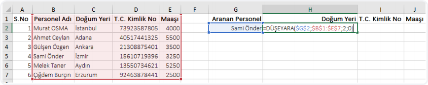
And our formula will look like this as you can see in the image.
=DÜŞEYARA($G$2;$B$1:$E$7;2;0)
DÜŞEYARA is the Turkish word for VLOOKUP. So in English it would be:
=VLOOKUP($G$2;$B$1:$E$7;2;0)

And when we drag our formula right, since we wrote 2 manually to the col_index_num argument, that part will always stay as 2.
Our aim here is to change the col_index_num argument by increasing 2,3,4 when we drag the formula right and to get the data in those columns.
Right at this moment comes the COLUMN function to our help.

What is the COLUMN function? How is it used?

The COLUMN function returns the column number of the given cell reference.
It is used in two ways.

When it is written as =COLUMN(), gives the number of the column of the cell in which it is written.
When it is written as =COLUMN(reference address) gives the number of the column of the cell stated as the reference address.

If you write the =COLUMN() formula into the E10 cell, since the E column is the 5th column in Excel, the formula will return the number 5.
Likewise, if you write the =COLUMN(B1) formula into the E10 cell, since the B column is the 2nd column in Excel, the formula will return the number 2.
Since we didn’t pin anything in the B1 cell address, when we drag the formula right it will change as C1, D1, E1. And this allows us to get the numbers 2,3,4,5.
Thanks to this, we will be able to get the data from the other columns in the table_array range.

You can see the sample formula below for the situation we want.

Our second method…

We will not use an auxiliary function in this method, but since the argument that will change will be col_index_num, we will try to get a result with the array in that part.
Which means that we will write the column index numbers we want to get as {2;3;4} and make it an array formula and make each one of these numbers transmitted to each column.

Here is how we’ll do it:

Edit the formula in the H2 cell like in the image.
Choose the field we will transmit the result of the formula to. (H2:J2)
Press F2 and get into the cell.
Press Ctrl + Shift + Enter and complete the formula entry.

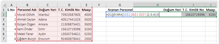
Being able to write the col_index_num we want into the col_index_num argument within {…..} curly braces will allow us to get the data in the columns we want and grant us with flexibility.

VLOOKUP FROM THE RIGHT

As you know, look ups are done from left to right all the time in Excel. Look ups can be from left to right in columns are in characters of a text.
And many functions have been created and released with the same logic. The VLOOKUP function is one of these functions.

As we have mentioned in the Working Conditions above, the lookup_value always has to be in the first column of the table_array in the VLOOKUP function. If it is not found, the formula returns the #N/A error.
By the way, this is not an “error” like we think it is, it is just a warning meaning that the looked up value does not exist in the table.
Getting an error when the data we look up is not in the first column of the range we have stated is a code related result of the VLOOKUP function.

Let’s have an example of this situation if you please.
If the cell range chosen for the table_array argument starts from the A column while looking for the personnel named Murat OSMA, an error will be returned since there will not be a personnel name in the first column of the field we have selected. This is completely normal.

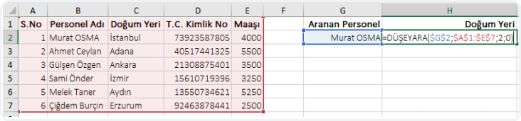
We can arrange this working style of the VLOOKUP function that causes us to get an error the way we want.
There are a few different methods for this too, but I will try to explain the easy one for you.

We have a function named CHOOSE.
This function requires an index_num and selecting arrays, i.e. data clusters.
The formula written in the image below is: =ELEMAN(1;C1:C7;B1:B7) [ELEMAN is the Turkish version of the CHOOSE function. Thus, in English it would be: =CHOOSE(1;C1:C7;B1:B7)]
We have written 1 as the index_num in the formula, and then chose each data range (arrays); first the C1:C7 range and then the B1:B7 range.
Since we wrote 1 into the index_num and choose the C1:C7 data range as the 1st data range, this formula will return the data in the C1:C7 range.
If we had written 2 into the index_num, it would have returned the data in the B1:B7 range.

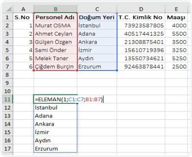
We get the data in the column we want when we state these index_num and arrays.
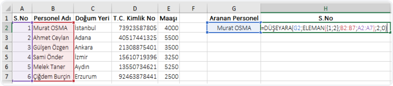
You see the formula you can use to prevent errors and get the data you want.
We state in which range the result should be by writing it in col_index_num within { … } in the index_num argument
by using the CHOOSE function in the table_array argument in the VLOOKUP function.
This way, if you write 1 into the col_index_num, you will get the result in the B2:B7 range and if you write 2, you will get the result in the A2:A7 range.

USING THE RANGE_LOOK UP ARGUMENT [TRUE – APPROXIMATE MATCH] (1)

We usually use the VLOOKUP function to get the data that matches exactly with the value we are looking for.
And 95% of the people who use this argument use the [range_lookup] argument as FALSE – Exact Match, i.e. 0.
So, what is this TRUE – Approximate Match?

When you look at the argument, it explains as:“the data in the first column of the table_array should be listed in an ascending order.”
So, when the [range_lookup] value is chosen as TRUE, sort the first column of the table_array before using the VLOOKUP.
If you don’t sort it, it is pretty likely to get the wrong data unless in an exceptional situation.
If the data in the table_array field is not sorted, if even if there is one that exactly matches, the #N/A error is returned.

When should you use TRUE – Approximate Match?

If the data in the table_array field is sorted, we can use the TRUE – Approximate Match.
If we are looking for a Numeric data and there is a number that matches with it, or there is no number that matches with it we can use it to bring the closest number to it.

Now, let’s have an example of this situation.
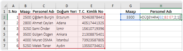
What we want to do in the formula written in the image below:
We want to find the Name of the Personnel of the Salary that is in the base of the number 3300 or numbers close to it.
For this action to give the correct result, keep in mind that the data in the first column of the table_array argument should be sorted.
The formula we write will give use the result of the name of the Personnel with the Salary of 3250 -since there is no one with the Salary of 3300 and this is the closest one-, so the name of Sami Önder.

VLOOKUP BY TWO OR MORE CRITERIA

We have used the VLOOKUP function to find a data in the table and then get the data from the column we wanted so far.
If we want, we can also get a result depending on multiple criteria.

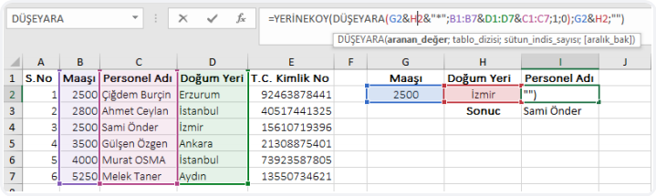
We have stated in the image below that we want to get this: Get the Name of The Personnel whose salary is 2500 and whose Place of Birth is İzmir.
And we used this formula for this:
=SUBSTITUTE(VLOOKUP(G2&H2&”*”;B1:B7&D1:D7&C1:C7;1;0);G2&H2;””)
We have used this technique here: We joined the Salary(Maaş in Turkish as you see in the image) and Place of Birth(Doğum Yeri in Turkish) in the lookup_value argument (G2&H2) and added &”*” at the end, and thus got to state that our conditions start with these.
And we have joined the ranges of Salary, Place of Birth and the Name of Personnel that we want to get as a result in the table_array argument.
Since we have joined the ranges we wanted to get and we were looking for with & in a single field, we have written 1 in the col_index_num argument.
We have written 0 for Exact Match in the range_lookup argument.
As a result, it returns us the 2500İzmirSami Önder text.
Lastly, when we say leave the data we write in the lookup_value argument blank in the text returned from the SUBSTITUTE function,
here will be the Personnel Name left Only.
This way, we got to find the data we were looking for by multiple criteria.

WHAT YOU SHOULD DO WHEN THE DATA TYPE YOU ARE LOOKING FOR AND THE DATA TYPE YOU FIND IS DIFFERENT?

Sometime even though a data should be numeric, it is determined as text because of the call style.
In this case, you might have realized that Excel warn you with green triangles and yellow warning symbol on the top left of these cells.
When you click that warning symbol, you will see the Number Stored as Text expression.
This explanation tells us that the data in the cell is a number but since the cell style is text, I store this number you have written as a text.

If the data type in the cell stated as lookup_value is a text,
the data type of the first column of the cell range we have stated as table_array must be text as well.
Or you can think of the opposite situation. To sum up: the types of the looked up and found data should be the same.
If they are not the same, the #N/A error is returned.
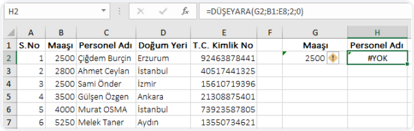
You can see the example about this in the image below. The formula used is:
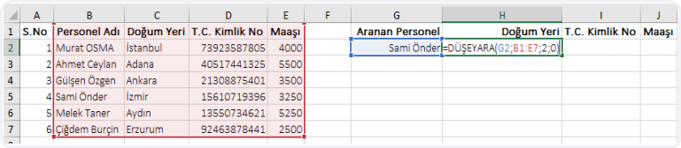
=VLOOKUP(G2;B1:E7;2;0)
Since the data type of lookup_value is text, and the data in the first column of the table_array is numbers, there is no match and the #N/A error is returned.

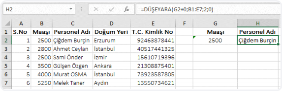
So, how do we solve this? It is very simple!

We can solve this problem by applying a mathematical operation that would turn the text stated as the lookup_value into a number.
The mathematical operation to be applied shouldn’t affect the existing number.
For example, if we use any mathematical operation like +0, *1, /1, ^1 or — (plus 1, multiply by 1, divide by 1, exponent 1, hyphen hyphen), we will get the result you can see below.
The formula used: =VLOOKUP(G2+0;B1:E7;2;0)

USE VLOOKUP INSTEAD OF WRITING NESTED IFS

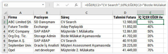
In some of our tables, for example when we want to calculate annual leave, we can write many nested IF function and find the solution that way.
But the VLOOKUP gives us the solution to solve this calculation faster and easier.
Now, let’s make the same calculation with nested IFs and then with VLOOKUP. You will see the difference.

Let’s assume that we have a table like the one below. We will determine different rations depending on the different processes. If we want to do it with nested If functions, we will have to write the formula long like this:

=IF(C2=”CV Search”;10%;IF(C2=”Bizde Mülakat Aşamasında”;20%;
IF(C2=”Aday Paylaşıldı”;40%;IF(C2=”Müşteride 1.Mülakatta”;50%;
IF(C2=”Müşteride 2. Mülakatta”;70%;IF(C2=”Müşteri Assessment Aşamasında”;80%))))))

We have shared this with the Turkish sentences so that you can see the cells in the table. However, the formula would be like this with the English translation of these sentences:
=IF(C2=”CV Search”;10%;IF(C2=”In the interview stage with us”;20%;
IF(C2=”The candidate has been shared”;40%;IF(C2=”In the 1st interview with the customer”;50%;
IF(C2=”In the 2nd interview with the customer”;70%;IF(C2=”The costumer is in the Assessment stage”;80%))))))

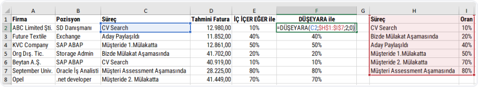
Whereas it would be way better to find the percentage ratio with the VLOOKUP function if we had a table of all processes and ratios.

Yeess…
If you have read, comprehended and applied everything so far, your are an EXPERT in VLOOKUP now. 👏🏻

You can share this post to help many people get informed and get Excel Training to use Excel more efficiently and productively. 👍🏻

GEOGRAPHY LINKED DATA TYPE

GEOGRAPHY DATA TYPE

There were always data types in Excel. But they were traditional data types like text and number. Stocks and Geography data types are unique because they are accepted as linked data types. Linked data types have a connection to an online data source. For now, linked data types are only Stocks and Geography. Microsoft plans to share more linked data types in the future with the feedback from the clients. We will be sharing the new linked data types here.

Office 365 users can access a lot of data of countries by clicking their names only. You will see the Geography linked data type in the data Types group of the Data menu. This features allows us to get and list a lot of indicators like flags, capitals, currencies, data ratios, populations, military power, president, average life time of the countries through http://data.worldbank.org/. It is possible to access more detailed information of countries with the link I gave you, and you can even download this data in the Excel, Csv and Xml format and use them in your reports.

It is enough to write the country name in the A column one under another and choose the Geography type.

DATA CART

First, we wrote the names of 5 countries and chose the Geography data type.
After the country name in the cell is turned into the Geography data type, an icon is seen in the cell.
Click the icon to view the cart. Cart shows a list of areas and related values.
There might be a lot of areas that you can view and work with depending on the data. If you click the icon next to the country name, you will see that you can get the flag of that country and a lot more information.

When you select a country in a cell, an option list called Add Data pops up next to it.
When you choose the information you want to get from that list, that information will be listed quickly next to it.

You can list a lot of information about the country or countries you select next to one other and turn them into a table like below. If you want, you can indicate the data you want to get for a country and then drag it down to list the data of all countries in the indicated area.

You can write =A2. to call the data in the related areas from the defined names with a formula.

When you right-click the countries, you can see the Show Cart option within Data Type in the menu. (Ctrl + Shift + F5) You can turn off the feature by converting the data into Text. You can cancel the Geography data type whenever you want like converting the tables into a range.

I hope this helps you.👍🏻
You can share this article with your friends and make it reach out to many people. Don’t forget: The more information is shared, the more valuable it gets.

coğrafya veri türü data type Excel file trickster msexcel office insider

HAVE YOU EVER SORTED WITH A FORMULA?

THE SORT FUNCTION

Hello everyone,

No doubt that one of the most frequently used functions in Excel is the Sort function.
This feature has 2 constants: A-Z and Z-A i.e. Ascending and Descending Sort.
We sort our data by certain field in pretty much all tables.
Have you ever tried to get this sorting action done with a formula?

WHAT DOES IT DO

You can easily sort columns or rows by the sort order you want in a different field from your mail table with the SORT function that is one of the dynamic array functions that are recently released after Office 365 .

SYNTAX

=SORT(array,[sort_index],[sort_order],[by_col])

There are 4 arguments in the function.
The first one is required, the next 3 arguments are optional.

Now, let’s take a look at what these arguments mean, i.e. what the function wants from us and what we will give it.

Argument	Description
array Required	The range, or array to sort
[sort_index] Optional	A number indicating the row or column to sort by
[sort_order] Optional	A number indicating the desired sort order; 1 for ascending order (default), -1 for descending order
[by_col] Optional	A logical value indicating the desired sort direction; FALSE to sort by row (default), TRUE to sort by column

USE OF THE FUNCTION

Choose the fields you want from your table and state by which column and order you will sort.
When you choose a field for the array argument only, the data is sort based on the Ascending order.
If multiple columns are selected in the array argument, the column by which the sorting will be done is chosen.
You can choose the Descending order in the sort_order argument if you want. If you don’ choose it, the sort is always Ascending.
In the by_col argument, you can sort by column i.e. from left to right. If not chosen, the sorting will always be from top to bottom.

Let’s have an example and see what happens when we choose the array argument only.

Now, let’s choose multiple columns and state the sort_index argument as well.

Since we didn’t use the sort_order argument in the formula below, prices are sorted from the lower to the higher. Now, let’s use the sort_order argument in the same function and see our data sorted from the higher to the lower.

Lastly, let’s sort the data from left to right and now from top to bottom.

We will be talking about the other New Dynamic Array functions in our next articles.
And then we will be able to get things done way easier by using these new functions together. LONG LIVE THE NEW DYNAMIC ARRAY FUNCTIONS!

See you in other articles, bye. 🙋🏻‍♂️
You can share this article and help a lot of people get informed as well. 👍🏻

Excel file trickster msexcel office insider sırala sırala fonksiyonu Sıralama SORT

EXCEL’S HISTORY (EXCEL FROM PAST TO TODAY)

EXCEL’S HISTORY (Excel from Past to Today)

Hello everyone,

I received a lot of questions like “Who found Excel, how was it created? It develops all the time, I wonder how the first version was…” in many of the trainings I gave in corporate companies.

As an answer to there questions, I have prepared the history of Excel and wanted to take the old users to a time travel that would make them say: “”Oh! What times…” And it will serve as an informative article for the new users.

Are you ready for the time travel? 👨🏻‍🚀

We met the first Excel as VisiCalc in 1978.
In 1978, Harvard Business School students Dan Bricklin ^{Father of the modern Excel}had to take on an analysis task for a case study. He had two alternatives to do that:

He would do it manually.
He would use a simple and unskillful computer program.

He thought that he didn’t have a better alternative and chose VisiCalc in the 1978 fall.
He programmed the first study and prepared the prototype of the concept he called VisiCalc. The first version of VisiCalc was a matrix of 4 columns and 20 rows.
It was not close to the electronic tables of our day but VisiCalc was still an accomplishment for that moment.

That was the first electronic table program and was published for Apple II at first.
It had skills like basic arithmetic operations, recalculating instantly and scroll bars.

1978 – VISICALC

1980 – SUPERCALC

1982 – MULTIPLAN

1983 – LOTUS 1-2-3

1985 – MICROSOFT EXCEL 1.0 (MAC)

1987 – MICROSOFT EXCEL 2.0 (WINDOWS)

1990 – MICROSOFT EXCEL 3.0

1992 – MICROSOFT EXCEL 4.0

1993 – MICROSOFT EXCEL 5.0

1995 – MICROSOFT EXCEL 7.0 (Excel 95)

1997 – MICROSOFT EXCEL 8.0 (Excel 97)

1999 – MICROSOFT EXCEL 9.0 (Excel 2000)

2001 – MICROSOFT EXCEL 10.0

2003 – MICROSOFT EXCEL 11.0 (Excel 2003)

2007 – MICROSOFT EXCEL 12.0 (Excel 2007)

2010 – MICROSOFT EXCEL 14.0 (Excel 2010)

2013 – MICROSOFT EXCEL 15.0 (Excel 2013)

2016 – MICROSOFT EXCEL 16.0 (Excel 2016)

2019 – MICROSOFT EXCEL 16.0 (Excel 2019)

2019 – MICROSOFT EXCEL 16.0 (Office 365)

Now I leave you alone with the 1992 Microsoft Excel introduction..

Well, I hope that you enjoyed this few-minute trip to the past.
You can share this post and take a few more people to the past as well. 👍🏻

Good bye.

Excel excelin tarihçesi file trickster msexcel office insider

SORT DATA WITH THE SORTBY FUNCTION

THE SORTBY FUNCTION

Hello everybody,

There are functions about sorting among the newly released dynamic array functions. They are:

SORT
SORTBY

We will be talking about the SORTBY function in this article.

WHAT DOES IT DO

With the SORTBY function that is one one the recently release dynamic array functions after Office 365, you can sort your table based on multiple columns/rows and sort order you want in a field without touching your table. Imagine suing the Sort feature we use a lot in Excel through the Custom Sort window. If we want to sort by multiple fields, we choose a column there and use one of the A to Z or Z to A options in the Order field and then choose the other field and choose the sorting order again. Thus, our table is sorted by the columns/rows and order we chose. Now we can do all this with one single function.

SYNAX

=SORTBY(array, by_array1, [sort_order1], [by_array2, sort_order2],…)

There are 3 arguments in the function.
The first two are required, the others are optional.

Now let’s take a look at what these arguments mean, i.e. what the function wants from us and what we will give it.

array

Required

The array or range to sort

by_array1

Required

The array or range to sort on

[sort_order1]

Optional

The order to use for sorting. 1 for ascending, -1 for descending. Default is ascendi

USE OF THE FUNCTION

the data range to be listed in the array argument.
the data range by which the sorting will be done based on which column/row first in the by_array1 argument.
the sort order is chosen in the sort_order1 argument. If it is not stated, the A to Z order is accepted.
you can continue by choosing a data range first and then sort order in the next optional array and orders.
you have to state at least one column/row in the by_array1 argument.

Let’s give an example and see what happens when only the optional arguments are chosen.

Now, let’s make the sort_order argument -1 and thus sort by Z to A .

SORT BY MULTIPLE FIELDS

We have sorted by one column and order so far. Now it is time to sort by multiple fields and orders. 😉 Let’s sort the Marka(Brand) field A to Z and then sort the Fiyat(Price) field Z to A and then change the sorting order of the Fiyat(Price) field and see the result.

SORT FROM LEFT TO RIGHT IN A HORIZONTAL TABLE

If you wish, you can sort the data in the field you’ve stated as an array by the stated array or order from left to right in a horizontal table. The important thing is to state the array to be returned, field to be sorted and the sorting order. The table will be sorted by the criteria you stated, doesn’t matter if it is vertical or horizontal.

See you in other articles, bye. 🙋🏻‍♂️
You can share this article and help a lot of people get informed as well. 👍🏻

Excel file trickster msexcel office insider sıralaölçüt yeni formül

THE TABLE FORMAT and ITS BENEFITS

In this article, we will be talking about the benefits of the table format of the data range in Excel. When we write titles and enter data under those title or when working on a prepared file we received, we say that we have prepared a table. But the data range we call a table is not a table for Excel yet. For it to be seen as a table, you need to format the data range as a table. At that point, it allows us to use a lot of features that table format allows us.

Now let’s take a look what we need to do before creating to table to use some features and how we do them after formatting as table. By the way, it would be very helpful to write the articles on our Blog when you have a chance. If you wish, you can read a detailed article on Office Support.

Choose Style for the Table Format

We can use this feature by choosing Format as Table in the Styles group in Home tab. Choose any cell on your data and click the Format as Table command and choose the table style you want. You will have turned your data into a table quickly. Don’t forget: Everything added to the page later is an object. An image, shape, chart, table, slicer etc. all of them are objects and a menu with features of objects added later is added to the Ribbon.

You can apply this feature easily with the shortcut keys.
Choose any cell on your data and turn your data into a table with the

CTRL + T

shortcut.

Now, let’s see what kind of features our data range gained with such a simple shortcut.

Benefits of the Table Format

When you choose a cell on the table and move upwards and downwards, the column titles will be the titles of your table. Thus, you don’t need to use the Freeze Top Row feature in the Freeze Panes field in the View tab.

A style is applied to our table automatically and each row is colored as dark and light successively one-by-one. And this creates a nice image.

When you keep entering data under the table or next to the table, your table gets longer and wider. And this enables the data we enter later to be included in the table and everything to be accepted as a whole.

Before applying the table format, when we want to get the 18% VAT in the Sum field written to the next column; we had to write the formula into a cell and drag it down first. If there are blank rows in between, we had do drag down again. But, when we format it as a table, it is enough to write the formula and press Enter for the formula to be applied on the whole column.

When we turn the data into a table, a menu named Table Design or just Design is created in the Ribbon. This menu contains the features that we can use for our table. One of the most important features is the Slicer feature that we are familiar with from the Pivot Table. This feature enables us to filter the area we want on our table with one click.

It allows us to add functions like sum, average, count, min, max easily when we filter on the table. You can take a look at the other Table Style Options.

When you create a Pivot Table from the data range, you have to choose Change Data Source most of the time when new data is added outside the field specified as the range. Considering that you add new data to your table every day, you will have to choose Change Data Source and specify the new data range all the time. But, when we turn our data into a table, the data we add under it or next to it will be accepted as a part of the table and is within the data range. Thus, it will be enough to Renew for the data to be reflected on the Pivot Table.

In the formulas, we get to specify the data range by writing the table’s name without having to choose the whole table.

We have seen a lot of positive features till now and we obtained them with CTRL + T only.

Big or small, we recommend you to use Format as Table while working with data.
This way, you will be able to use the features above that will make you gain visualization and speed.

Convert to Range

Lastly, when you want to convert your table to data range again, you have two options.

By choosing Convert to Range in the Table Design or Design menu.
By right-clicking a cell on the table and choosing Convert to Range from Table.

I hope that this was a helpful article for you.
You can share this article with your friends and help a lot of people get informed as well.

Good bye. 👍🏻

Excel file trickster msexcel office insider table table style tablo tablo biçim

CONCATENATE vs TEXTJOIN

Hello everybody!

In this article, I invite you to say goodbye to the old CONCATENATE function that when we wanted to add a space or any other character while concatenating the data, obliged us to do it one by one and thus that was very laboring, and say welcome to a more efficient function. If you need to join the data in multiple cells and add characters like a space, comma, semi colon, and hyphen; there is just one function that you need to use and that is the TEXTJOIN function.

WHAT DOES IT DO

Like I mentioned above, you don’t need to click cells one by one and use an expression like ;” “; to add a space in between each time or a statement like & ” ” & when joining with the & character in the textjoin function. It joins each cell in the selected cell range by adding the slicer we’ve indicated. This way, we can join the data in hundreds of cells easily as a text.

SYNTAX

TEXTJOIN(delimiter, ignore_empty, text1, [text2], …)

There are 3 main arguments in the function.

These 3 main arguments are required, the other arguments are optional.Now let’s take a look at what these arguments mean, i.e. what the function wants from us and what we will give it.

delimiter (required)	A text string, either empty, or one or more characters enclosed by double quotes, or a reference to a valid text string. If a number is supplied, it will be treated as text.
ignore_empty (required)	If TRUE, ignores empty cells.
text1 (required)	Text item to be joined. A text string, or array of strings, such as a range of cells.
[text2, …] (optional)	Additional text items to be joined. There can be a maximum of 252 text arguments for the text items, including text1. Each can be a text string, or array of strings, such as a range of cells.

WORKING CONDITIONS

If the resulting string exceeds 32767 characters (cell limit), TEXTJOIN returns the #VALUE! error.
It came with Microsoft Excel 2019. If you are using and older Office version, you will get the #NAME? error and thus not be able to use this function.
If you Office 2019 or Office 365, you can easily use this function.

USING THE FUNCTION

After we write the function name, we specify the delimeter. And then we will choose how it should behave about the possible blank cells in the cell range. And in the last arguments, we choose the cell range to be joined. Now, let’s take a look at its use together.

In the example below, we join the data between the A and G columns with a semi colon in between them.

As you see, it is as easy as that to join a multiple cell range in a single text with any character between them.

See you in another articles, bye. 🙋🏻‍♂️
You can share this post with your friends and help them get informed as well.👍🏻

Excel file trickster MetinBirleştir msexcel office insider Office365 textjoin

IDEAS

In this article, I will be talking about the Ideas feature of Excel.

Explore your data in more detail with Ideas.

The Ideas button -one of the new features- explores the order within your data and offers smart and custom ideas by using that.
Ideas in Excel empowers you to understand your data through natural language queries that allow you to ask questions about your data.
Simply click a cell in a data range, and then click the Ideas button on the Home tab.
Ideas in Excel will analyze your data, and return interesting visuals about it in a task pane.

Creates dozens of artificial intelligence analysis and reports from the data in your table for you.

On which data do Ideas work?

Ideas work best when data is formatted as an Excel table with a single title row on top.

Here is an example:

Ideas works best with clean, tabular data.

Here are some tips for getting the most out of Ideas:

Ideas works best with data that’s formatted as an Excel Table. To create an Excel Table, click anywhere in your data and then press Ctrl+T.
Make sure you have good headers for the columns. Headers should be a single row of unique, non-blank labels for each column. Avoid double rows of headers, merged cells, etc.
If you have complicated, or nested data, you can use Power Query to convert tables with cross-tabs, or multiple rows of headers.

Didn’t get Ideas?

Here are some reasons why Ideas may not work on your data:

Ideas doesn’t currently support analyzing datasets over 1.5 million cells. There is currently no workaround for this. In the meantime, you can filter your data, then copy it to another location to run Ideas on it.
String dates like “2017-01-01” will be analyzed as if they are text strings. As a workaround, create a new column that uses the DATE or DATEVALUE functions, and format it as a date.
Ideas can’t analyze data when Excel is in compatibility mode (i.e. when the file is in .xls format). In the meantime, save your file as an .xlsx, .xlsm, or xslb file.
Merged cells can also be hard to understand. If you’re trying to center data, like a report header, then as a workaround, remove all merged cells, then format the cells using Center Across Selection. Press Ctrl+1, then go to Alignment > Horizontal > Center Across Selection.

We’re always improving Ideas

Even if you don’t have any of the above conditions, we may not find a recommendation. That’s because we are looking for a specific set of insight classes, and the service doesn’t always find something. We are continually working to expand the analysis types that the service supports.

Here is the current list that is available:

Rank: Ranks and highlights the item that is significantly larger than the rest of the items.

Trend: Highlights when there is a steady trend pattern over a time series of data.

Outlier: Highlights outliers in time series.

Majority: Finds cases where a majority of a total value can be attributed to a single factor.

See you in other articles, bye. 🙋🏻‍♂️

You can share this post with your friends and help them get informed as well.👍🏻

Excel fikirler file trickster ideas msexcel office insider

Office Insider – What Happened in July?

NEW FEATURES/FIXES

You can find and follow all monthly Office insider new features and fixes (updates) on our blog. 👍🏻 Officer insider gets updates and new features regularly. It is important to follow these Office insider updates and use them in terms of increasing your knowledge. Now let’s take a look at what kind of changes happened in Office insider in the month of July.

July 06, 2020

Outlook

Create polls in email quickly and easily

Easily create a poll, collect votes, and view results within an email.

Learn more

New room finder

Search for conference rooms by different capabilities.

Learn more

Notable fixes

We fixed an issue where Outlook would hang if there were over 130 recipients on the To line, and we also improved the performance of rendering the text.
We fixed an issue in the To Do Bar where events that spanned more than two days displayed the same end time for all subsequent days.
We fixed an issue that caused users of Outlook to see their message list stop updating for several minutes after using shared calendars.

Excel

Notable fixes

We fixed an issue where data model tables created in certain versions of Excel could not be seen in ‘Table Preview’ even though the query associated with the table had not been edited.
We fixed an issue where disabling Ignore Relative/Absolute references in the Define Name Apply Names dialog would cause formulas not to work.
We fixed an issue where clearing an advanced data filter could lose table formatting.
We fixed an issue where the full path of an embedded PDF document would show in the document caption rather than just the filename.
We fixed an issue where after disabling the Wolfram cloud connector and then saving and re-opening an Excel workbook could result in a crash.
We fixed an issue where booting Excel with the Solver add-in enabled would result in a crash.

PowerPoint

Notable fixes

We fixed an issue where pasting HTML to a text area on a slide would instead get pasted into a text box created at the top of the slide.
We fixed an issue where selecting all slides in Presenter View, then exiting Presenter View using Alt+Tab and returning to the slide show, and clicking ‘End Show’ would result in an unhandled exception.

Word

Notable fixes

We fixed an issue during co-authoring mode when there is a merge conflict, and the user has already chosen to discard changes. We no longer display the option to save or discard changes.
We fixed an issue that, when attempting to save a file containing a macro under a new name, would cause it to be saved with a .docx extension and the filename WRO0004.docx regardless of what the user entered, which rendered the document unusable.

Project

Notable fixes

We fixed an issue where Project may crash when opening certain XML files.
We fixed an issue where you couldn’t open a Project file from a SharePoint document library if the library were in modern mode.
We fixed an issue where projects couldn’t be opened in the Project desktop client from the Project Web App if the URL ended in .com.

July 10, 2020

Word

Notable fixes

We fixed an issue where Word would stop responding after pasting some text and an image in a comments box.
We fixed an issue where the New comment button would be disabled after deleting the last comment.

Outlook

Notable fixes

We fixed an issue where the Allow Forwarding option was missing from the shared calendar meeting Response Options if Download Shared folder was not checked.
We fixed an issue that would display the print button in a disabled state even though the user had the appropriate print permissions.

Project

Notable fixes

We fixed an issue where if you tried to save a PDF/XPS from Project to a SharePoint document library, nothing would happen.

July 15, 2020

Excel

Sheet View

You can now sort and filter your Excel file while collaborating with others with Sheet View. This new feature prevents you from being impacted by other user’s sorts and filters while coauthoring the document.

Learn more >

LET – Names in formulas for Excel

The LET function allows you to name, and then use a calculation or value in your formulas, and increase both readability (by giving context to others) and performance (by reducing the number of times an expression is calculated). It’s names but on a formula level.

Learn more >

Create a PivotTable from Power BI datasets

You can create PivotTables in Excel that are connected to datasets stored in Power BI with a few clicks. Doing this allows you get the best of both PivotTables and Power BI.

Learn more >

Speedy SUMIFS

Have you ever used SUMIFS, AVERAGEIFS, COUNTIFS, MAXIFS, and MINIFS as well as their singular counterparts SUMIF, AVERAGEIF, COUNTIF, MAXIF, and MINIF to aggregate lots of data? In this update of Excel, you’ll notice these calculations are noticeably faster.

These functions now create an internal cached index for the column range being searched in each expression. This cached index is reused in any subsequent aggregations that are pulling from the same range. The effect is dramatic: For example calculating 1200 SUMIFS, AVERAGEIFS, and COUNTIFS formulas aggregating data from 1 million cells on a 4 core 2 GHz CPU that took 20 seconds to calculate using Excel 2010, now takes 8 seconds only, on Excel M365 2006.

PowerPoint

Faster playback comes to Microsoft Stream videos

Microsoft Stream lets people in your organization upload, view, and share videos securely. You can share recordings of classes, meetings, presentations, training sessions, or other videos that your team needs. We previously enabled Stream as one of the supported online video sources in PowerPoint. Over the last few months, we’ve made significant performance improvements to the video playback experience. Now you’ll experience faster playback of Stream videos in your PowerPoint presentations.

Outlook

Create polls in email quickly and easily

Easily create a poll, collect votes, and view results within an email.

Learn more>

Quickly reopen items from previous session

We added an option to quickly reopen items from a previous Outlook session. Whether Outlook crashes or you close it, you’ll now be able to quickly relaunch items when you reopen the app. This feature is on by default. To turn it off, go to Options > General > Start up Options.

Learn more>

Disable @ mentions

Do you find the @ mention picker more annoying than useful? Now you can turn it off. Find the option under the new checkbox under File > Options > Mail > Send Messages in Outlook.

Transfer Outlook settings automatically

Outlook will now store/retrieve settings from the cloud, so when you set up a new Windows device, your settings will be loaded automatically based on your Office identity.

Store your signatures in the cloud

Signatures now follow your account across Windows devices. Set up your account once, and new installations of Outlook will have your signatures.

July 17, 2020

Excel

Notables fixes

We fixed an issue where any time a pivot chart with hidden leader lines was saved and reopened, the leader lines would become visible.
We fixed an issue where charts were not always updated as expected when “ForceFullCalculation” was enabled via VBA for the workbook.

Word

Notable fixes

We fixed an issue where the Show Markup command was disabled when the focus was on a comment text box.
We fixed an issue where the Editor command was disabled when the focus was on a comment text box.
We fixed an issue in custom XML that state of comments may be lost when opening the document.

Outlook

Notable fixes

We fixed an issue around creating multiple profiles in Outlook from the same email domain.
We fixed an issue that caused the lock icon to fail to display in the header of S/MIME encrypted messages.
We fixed an issue that caused attachments to get stripped from S/MIME messages when sending as unencrypted.
We fixed an issue that caused users to be unable to save OneDrive attachments from outside their tenant to their local computer when selecting the Save option on the security dialog.
We fixed an issue that cause recipients to be unable to save rights protected messages even when the save as permission was granted by the sender.
We fixed an issue that caused plain text S/MIME messages to become garbled when sending.
We fixed an issue that caused attachments to become corrupted when sending an S/MIME email unencrypted.
We fixed an issue that caused the labels for some Advanced Search options to be truncated in some languages.

Project

Notable fixes

We fixed an issue where the tasks listed in the Task Board view were not in sync with those in the Assign Resources dialog.
We fixed an issue where if you copied and pasted a task that had multiple dependencies, not all dependencies were copied correctly.

Office

Notable fixes

We fixed an issue where after the user opened a new app window from the taskbar and created a new blank document, additional files were created.
We fixed an issue where if a user was editing a document but had lost permissions, we were not notifying the user that they had to re-authenticate.

July 24, 2020

Visio

Create charts with data in worksheet

Visio Data Visualizer can help users convert their excel data into high quality flowcharts, swim line diagrams, and org charts. These diagrams can be viewed in Visio, downloaded as images, printed, etc. They can also be opened in Visio for richer editing capabilities.

Learn more >

Word

Notable fixes

We fixed an issue where an occasional hang occurred while opening HTML files.
We fixed an issue where the Specific People option for Track Changes was disabled.
We fixed an issue where the placeholder text in the Search edit box would overflow if the application window was resized to a small dimension.

OneNote

Notable fixes

We fixed an issue where the placeholder text in the Search edit box would overflow if the application window was resized to a small dimension.

July 31, 2020

Excel, PowerPoint, Word and Outlook

Insert Apple photos into Office easily

We’re happy to announce inserting Apple photos into Office is easier than ever. You can now insert pictures taken with your iPhone or iPad into Word, Excel, PowerPoint, and Outlook on Windows! We had heard from many of you that converting these files was too time consuming, so we’ve simplified the process.

Learn more >

Excel, PowerPoint, Word

Notable fixes

We fixed an issue where a copy of an image with a radial gradient fill did not match the original.

Excel

Notable fixes

We fixed an issue where if the order of a chart series was changed, the corresponding checkbox aligned with the series was not reordered along with the series.

PowerPoint

Notable fixes

We fixed an issue where the Forms button in PowerPoint did not allow the creation of Forms when access to the Office Store was not permitted.

Word

Notable fixes

We fixed an issue where if a comment was added to track a change, the revisions pane would unexpectedly open.
We fixed an issue where links to documents were not being inserted to the comments box via the Insert > Link dropdown.
We fixed an issue where the hyperlink count in the VBA hyperlinks collection was not iterating correctly after adding an image containing a hyperlink.

Outlook

Notable fixes

We fixed an issue that caused users to be unable to add a signature when replying to a digitally rights managed message from an inspector window when the user did not have Owner permissions on the message being replied to.
We fixed an issue that was causing Outlook to fail to display line breaks properly in markdown content.

Access

Notable fixes

We fixed an issue where trying to run certain queries have previously produced the error message “Query is too complex.”

Project

Notable fixes

We fixed an issue where for a SharePoint tasks list, the ribbon buttons on the second tab may be disabled.

We compiled all the new features and fixes in July in Office insider. Hope to see you in our other articles, bye bye. 🙋🏻‍♂️

You can share this article with your friends and family to help them get information about Office insider updates released in the month of July. 👍🏻

file trickster office insider Office365

Office Insider – What happened in August?

NEW FEATURES/FIXES

📅August 07, 2020

PowerPoint

Notable fixes

We fixed an issue where users were seeing the ribbon/title bar not being displayed under certain conditions.

Outlook

Notable fixes

We fixed an issue where the user account attributes in Active Directory for “otherTelephone” and “otherHomePhone” were not mapped to the corresponding Outlook LDAP attributes.

📅August 11, 2020

Word

Explore modern comments

Add comments to objects, @mention colleagues, and resolve comment threads for a better collaboration experience.

Word’de modern açıklama ekleme

Learn more >

Outlook

Delete messages

Delete messages and conversations in CML view.

📅August 14, 2020

Excel

Notable fixes

We fixed an issue where if a user typed a formula name including the parenthesis and invoked help via F1, the help topic specific to that formula would not be displayed.
We fixed an issue where macro links to buttons were broken after restoring the file to an older version of Excel.

Word

Notable fixes

We fixed an issue where the bullet picture icon didn’t display correctly.

Outlook

Notable fixes

We fixed an issue where the Meeting page would continue to be displayed after the user switched tabs from the Meeting page to the Scheduling Assistant page.

We compiled all the new features and fixes in August in Office insider. Hope to see you in our other articles, bye bye. 🙋🏻‍♂️

You can share this article with your friends and family to help them get information about Office insider updates released in the month of August. 👍🏻

file trickster office insider Office365