The CONCATENATE function

The Concatenate function concatenates texts in different cells and allows you to write them in one single cell. Texts can be edited in a very flexible way with the Concatenate formula.

In this manner, you can freely change any field you want in the formula and get the desired result.

The arguments of the formula consist of successive textual expressions.

=Concatenate(text1, text2,…)

You can select the texts to be concatenated from the related cells one-by-one.

In the example bellow, the address is created by concatenating the Strict, Street and Number. When the A2, B2, and C2 cells are concatenated directly, it created the MerkezAyazma37 result.

To see a more familiar result like Merkez Strict Ayazma Street Number:37 (this is the Turkish way of writing an address), what can we do?

You can write textual expressions like “Street”, “Strict” into the formula with the long method.


*When you need to write a text with the keyboard into the formula, you need to write it into a double-quote (“ ”). Using texts in ” ” in Excel is pretty strict.

A more efficient method for it to be reusable, editable and controlled centrally is to write strict, street, number information into a cell and use that cell as a reference.

Click here to take a look the the details of the Concatenate formula.

In addition, it to possible to concatenate without using a function. You can use the & symbol as a concatenation operator. It works similar to the concatenate function and allows you to concatenate the texts directly.

We have learned how to concatenate texts above. In addition to this, we might want to separate concatenated texts as well.

You can separate texts written in one cell into separate cells with the Convert Text to Columns function. So, it works the opposite way of the Concatenate function. Click here to read our article about Convert Text to Columns.

XLOOKUP: THE GAME CHANGER

THE XLOOKUP FUNCTION

Last you on August 29, two new important functions were announced: XLOOKUP and XMATCH. In this article, we will be talking about what the XLOOKUP function is, when and how to use it. When you start using this function, you will just not be able to let it go.

I want to mention a few things about VLOOKUP first: as you know, the VLOOKUP function was indispensable for many users, even those who didn’t know wanted to learn it. And even in the 7 Most Used Excel Functions presentation Microsoft prepared, the first function is VLOOKUP.

As dispensable as it is for some users, it was useless for some others. Because VLOOKUP required some conditions to run and the function returned us the first match it found. On top of that, it decreased Excel’s performance since it could cause unnecessary calculation in the stated table range. It is the function for those who have unique data, but in a table with duplicate data -i.e. recurring data-  it wasn’t very useful since it didn’t give us all the records. Of course, there are some methods to list all the records, but you either had to solve the issue by using auxiliary columns or list all the records with the Array Formula.

LONG LIVE THE DYNAMIC FUNCTIONS!

Fortunately, in September 25, 2018 the new dynamic array functions were announced and we got to breathe a sigh of relief. After waiting for such a long time, now the new function will be able to return a whole array instead of returning just one single result.

Instead of writing an Array Formula that was known as “MULTIPLE VLOOKUP” by everyone, we can list all the records of a data with the FILTER function easily. *We will be talking about the details in its own article. (Here are the article links of Microsoft, you can take a look.)


With the release of the XLOOKUP function, old functions like VLOOKUP and HLOOKUP are not needed anymore. And also, as they get into more detail and design what they can do, it seems like we will not need these functions:
VLOOKUP > HLOOKUP > INDEX > MATCH > OFFSET > IFERROR(VLOOKUP).. what else do you want?!👏🏻


Just one formula can:

  • Look up both horizontally and vertically,
  • Bring the first or last record, find the data considering the wildcard characters,
  • Bring the data we want on the left without a condition like the lookup_value has to be in the first column of the table_array in the VLOOKUP function,
  • Bring approximate vales in  certain range like the TRUE option in the range_lookup argument,
  • Allow you to say write this if no data is found without the need to use the IFERROR formula,
  • Find the most approximate lowest or highest value if there is no exact match.
  • And it offers all these in a way more faster way than before.

Enough with all the details, let’s see what this function does. 👍🏻


THE XLOOKUP FUNCTION SYNTAX


=XLOOKUP(lookup_valuelookup_arrayreturn_array, [if_not_found], [match_mode], [search_mode]

There are 6 arguments in this function.
The first 3 are required, the last 3 are optional.

Now let’s take a look at what these arguments mean, i.e. what the function wants from us and what we will give it.

Argument

Description
lookup_value

Required

The lookup value
lookup_array

Required

The array or range to search
return_array

Required

The array or range to return
[if_not_found]

Optional

Where a valid match is not found, return the [if_not_found] text you supply.

If a valid match is not found, and [if_not_found] is missing, #N/A will be returned.

[match_mode]

Optional

Specify the match type:

0 – Exact match. If none found, return #N/A. This is the default.

-1 – Exact match. If none found, return the next smaller item.

1 – Exact match. If none found, return the next larger item.

2 – A wildcard match where *, ?, and ~ have special meaning.

[search_mode]

Optional

Specify the search mode to use:

1 – Perform a search starting at the first item. This is the default.

-1 – Perform a reverse search starting at the last item.

2 – Perform a binary search that relies on lookup_array being sorted in ascending order. If not sorted, invalid results will be returned.

-2 – Perform a binary search that relies on lookup_array being sorted in descending order. If not sorted, invalid results will be returned.


In the few examples below, you can see what you need to write when there is the first record and last record is not found of the looked up data and how to use it when looking up with wildcard characters.


Let’s have an example of the Match Mode argument with exact match or highest and lowest options.


So far we got the data from the column we wanted by looking up in the column just like in VLOOKUP. Now, let’s use this function like HLOOKUP.


Now, let’s have a 2 dimension look up. Let’s match based on both the Product name and Month, and find the data in the intersecting cell. Users who know how to use the INDEX and MATCH functions usually do the matching we are about to the with the INDEX + MATCH + MATCH formulas. Now, let’s see how it is done with XLOOKUP.


Lastly, let’s compare the VLOOKUP and XLOOKUP function while finding the same data. At first, you will see that you get the same result, but when we add or delete a column, the VLOOKUP function will give us an incorrect result. But the result will not change in the XLOOKUP function. The reason is this: Since we write the column number that we want to get manually in VLOOKUP, the col_index_num stays stable but the column of the data changes and it returns an incorrect result. And in XLOOKUP, it doesn’t matter how many columns you add or delete, since we stated the column we want, that column changes dynamically and returns the correct result without producing any errors.


You can see the result in this example.

I hope this was helpful..  👍🏻
You can share this post and help many others get informed as well. Keep in mind that information gets more valuable when it is shared.

Excel Shortcuts1

It is possible for you to get to your destination the fastest way when you use shortcuts. But when you get support from the Navigation, it is probable that you will taking the fastest and traffic-free way.

We, as Office lecturers, offer you the most special and functional Excel shortcuts below for you to get to the result you want faster and in an optimum way.

Move Cells Between Pages

The Alt Shortcut:
It is enough to drag and leave while pressing the Alt key to move cells. This way, you can move cells to the page or location you want.

Create a New Line in the Cell

Alt & Enter Shortcut:
You can write texts one under the other or create articles in a cell in Excel just like in Word. It is enough to press the ALT and ENTER keys to move onto the next line in the cell.

Fastest Way to Create a Chart

Alt & F1 Shortcut:
It is the shortcut that allows you to create a chart the fastest way possible.
Select a field in the list you want to create a chart from and then press the Alt and F1 keys. A chart like the one below will be created quickly.

Navigate in the Page Fast

Ctrl & Arrow Keys:
You can quickly navigate in your list with the Ctrl & Arrow keys. You can reach the last full cell in your list. You can change the direction with the arrow key you want while pressing the Ctrl key.
*This is a general shortcut, you can even use it to navigate between texts while writing a text on your device.

Select Step by Step in the Page

Shift & Arrow Keys:
Allows you to select the cells in your list one by one. You can change your selection with the arrow key you want while pressing the Shift key.
*This is a general shortcut. You can even use it to select texts while writing a text on your device.

Bulk Selection in the Page

Ctrl & Shift & Arrow Keys:
You can select one by one with the Shift key, and if you want to make this action faster you can add the CTRL key. This way you can select way faster!
*This is a general shortcut. You can even use it to select texts while writing a text on your device.

Experience the easiness of adding and deleting a column/row quickly.

Ctrl & –  Shortcut and Ctrl & + Shortcut

You can delete columns/rows with the Ctrl & – keys,  and add columns/rows with the Ctrl & + keys.

Make the Cells Writable

F2 Shortcut:
We usually double-click the cell in order to write something in it. But it is enough to use the F2 shortcut instead of this.
*This is a general shortcut. You can even use it to change the name of a file on your device.

Enter Data to All Selected Cells

Select the cells you want to enter the data to.
Don’t click anything else once you are done selecting. Write the text you want directly.
Press the Ctrl & Enter keys for the text to be distributed to all cells.

The Fastest Way to Create a Table in Excel

Ctrl & L Shortcut:

Repeat the last action!

F4 Shortcut:
Allows you to repeat your last action.

For example, highlight the A1 cell with green and press the F4 key after clicking the B1 cell. You will see that the B1 cell will be highlighted with green as well! Since the previous action is repeated every time, you can just keep doing this with F4 forever!

It allows you to pin a cell while writing a formula. There are 4 different ways ($A$1 , A$1 , $A1, A1) to use this feature which is also known as Cell Reference Styles.

*Note: You might need to use the fn key (depending on your computer) to use the function keys with F like F1 and F2.


A combination of little clicks and keys can accomplish great things!

EVERYTHING ABOUT THE VLOOKUP FORMULA

The VLOOKUP Function

Hello everybody,

As you can understand from the title, this article will be pretty long.
If you want to become an expert in the VLOOKUP formula, you can read this article till the end and apply it.

It is a function that everybody has heard of, everybody wants to learn and that everybody uses in Excel. We use the VLOOKUP function to find a value in the table.
Let’s explain it a bit: we use the VLOOKUP function when we search a data in a table or data range and want to get data from a column that corresponds to that data. For example: let’s assume that you have a personnel salary table. In one cell there is the personnel name, you can search your employee’s name and find out the salary they get easily.

SYNTAX

VLOOKUP (lookup_value, table_array, col_index_num, [range_lookup])

To express how the VLOOKUP function works simply:

=VLOOKUP (look for this; look in this table; if you find it bring me the one in the 2nd column; [TRUE – Approximate Match / FALSE – Exact Match])

Now let’s take a look at the arguments this function wants from us.

Argument name Description
lookup_value    (required) The value you want to look up. The value you want to look up must be in the first column of the range of cells you specify in the table_array argument.

For example, if table-array spans cells B2:D7, then your lookup_value must be in column B.

Lookup_value can be a value or a reference to a cell.

table_array    (required) The range of cells in which the VLOOKUP will search for the lookup_value and the return value. You can use a named range or a table, and you can use names in the argument instead of cell references.

The first column in the cell range must contain the lookup_value. The cell range also needs to include the return value you want to find.

Learn how to select ranges in a worksheet.

col_index_num    (required) The column number (starting with 1 for the left-most column of table_array) that contains the return value.
range_lookup   (optional) A logical value that specifies whether you want VLOOKUP to find an approximate or an exact match:

  • Approximate match – 1/TRUE assumes the first column in the table is sorted either numerically or alphabetically, and will then search for the closest value. This is the default method if you don’t specify one. For example, =VLOOKUP(90,A1:B100,2,TRUE).

  • Exact match – 0/FALSE searches for the exact value in the first column. For example, =VLOOKUP(“Smith”,A1:B100,2,FALSE).

Working Conditions

  • When the required arguments are not entered, the function doesn’t work.
  • If the range_lookup optional argument is not entered, TRUE- Approximate match is considered as default.
  • The lookup_value always has to be on the far left (in first column) of the selected/indicated table array. But this situation can be overcome by writing different functions in VLOOKUP. (We will see this below.)
  • If the lookup_value is not found on the left of the table_array, #N/A error is returned.
  • If there is a multiple number of the data written into the lookup_value argument in the range indicated in the table_array argument, this function returns the record of the first data it found
  • it is not checked if the text written into the lookup_value argument is with uppercase or lowercase.
  • when a numeric data is written into the lookup_value argument, if the data type stated as table_array in the first column is text, #N/A error is returned. the same condition is valid in the opposite condition.
  • if a smaller number than 1 or a bigger number than the column number in the indicated table range or a text is written into the col_index_num  argument, #VALUE! error is returned.
  • when a column is deleted from the field stated as table_array, #REF! error is returned.
  • 1 and 0 can be written instead of TRUE and FALSE in the range_lookup argument.
  • If TRUE – Approximate Match is chosen, the table assumes that the first column will be sorted by number or alphabetically and looks for the most approximate value on the base. If you don’t specify a method, this method is used as default.
  • If FALSE- Exact Match is chose, if there is a value that is exactly the same with the data you have stated in the lookup-value argument is look for in the first column of the table_range.


THE BASIC USE OF THE VLOOKUP FUNCTION

You see a search sample suitable with the basic language and working conditions of the VLOOKUP function in the image below.

We have said that if you find the name Sami Önder in the B column which is the first column in the B3:D9 cell range , bring the data in the 3rd column of the selected range.

We have mentioned that we can write 0 instead of FALSE. With this FALSE expression, it i checked if there is an exact Sami Önder in the B column.


USING WILDCARD CHARACTERS

We can get the same result without having to write the full name we are looking for on the same table by using a wildcard character after writing the name only. Let’s brush up on the Wildcard Characters that we can use in Excel.

We have 3 different Wildcard characters.

Use

To find
? (question mark) Any single character
For example, sm?th finds “smith” and “smyth”
* (asterisk) Any number of characters
For example, *east finds “Northeast” and “Southeast”
~ (tilde) followed by ?, *, or ~

A question mark, asterisk, or tilde
For example, fy06~? finds “fy06?”


The asterisk and question mark act as complementary character when it is in the beginning or end of a text in the lookup_value argument of the VLOOKUP function.
And ~ only limits the other wildcard characters by preceding them.

If the wildcard character precedes the text, it implies that the text ends with that. For example: *ali (if it ends with ali)
If the wildcard character is at the end of the text, it implies that the text starts with the. For example: ali* (If it starts with ali)
If the wildcard character is both in the beginning and at the end of the text, it implies that the texts contains that. For example: *ali* (if the text contains the word ali)
here is an example for the question mark: when you write ?ali, it means that there is a character (text, numbers or symbols) before the word ali.
You can analyze this image as an example of the situation I have mentioned. ‘=F4&”*”


METHODS OF GETTING DATA FROM MULTIPLE COLUMNS

All Functions in Excel -except for the recently added dynamic array functions- return only one result.
When we get a result with the VLOOKUP formula, we might want to get the other data in the table by dragging the formula right.
Instead of writing the formula over and over again for each column, we can get data from the others column in the field we have stated as table_array when we drag the cell we have written the formula in right after adding a function to the col_index_num  function that would change it as dynamic.
We can execute this action with a few methods. Now, let’s analyze these methods.

Our first method..

Let’s assume that we have a table like the one here.
We will get the data in the I.D. Number and Salary fields when we write the Name of the Personnel and drag it right.


We will have to write our formula correctly to execute an action like that.
And by correctly I mean using the cell styles correctly.
Which mean will we pin the cells while selecting the cell or cell range or not, or are we going to pin the row or column only?
As an answer to these questions, we have to write the $ (dollar) symbols in the direction it is supposed to be when we select the cell.
And then we will have to use a function that would allow us the make the col_index_num  part dynamic.

Well, let’s start.

While selecting a cell in the formula, we have to think about the pinning issue we have mentioned.
Since the place of the cell in which we write the Name of the Personnel is stable, we press F4 and pin it.
And since the place of the cell range we selected for the table_array argument, we press F4 again and pin that cell range as well.
And our formula will look like this as you can see in the image.
=DÜŞEYARA($G$2;$B$1:$E$7;2;0)
DÜŞEYARA is the Turkish word for VLOOKUP. So in English it would be:
=VLOOKUP($G$2;$B$1:$E$7;2;0)

And when we drag our formula right, since we wrote 2 manually to the col_index_num argument, that part will always stay as 2.
Our aim here is to change the col_index_num argument by increasing 2,3,4 when we drag the formula right and to get the data in those columns.
Right at this moment comes the COLUMN function to our help.


What is the COLUMN function? How is it used?

The COLUMN function returns the column number of the given cell reference.
It is used in two ways.

When it is written as =COLUMN(), gives the number of the column of the cell in which it is written.
When it is written as =COLUMN(reference address)  gives the number of the column of the cell stated as the reference address.

If you write the =COLUMN() formula into the E10 cell, since the E column is the 5th column in Excel, the formula will return the number 5.
Likewise, if you write the =COLUMN(B1) formula into the E10 cell, since the B column is the 2nd column in Excel, the formula will return the number 2.
Since we didn’t pin anything in the B1 cell address, when we drag the formula right it will change as C1, D1, E1. And this allows us to get the numbers 2,3,4,5.
Thanks to this, we will be able to get the data from the other columns in the table_array range.

You can see the sample formula below for the situation we want.


Our second method…

We will not use an auxiliary function in this method, but since the argument that will change will be col_index_num, we will try to get a result with the array in that part.
Which means that we will write the column index numbers we want to get as {2;3;4} and make it an array formula and make each one of these numbers transmitted to each column.

Here is how we’ll do it:

  • Edit the formula in the H2 cell like in the image.
  • Choose the field we will transmit the result of the formula to. (H2:J2)
  • Press F2 and get into the cell.
  • Press Ctrl + Shift + Enter and complete the formula entry.

Being able to write the col_index_num we want into the col_index_num argument within {…..} curly braces will allow us to get the data in the columns we want and grant us with flexibility.


VLOOKUP FROM THE RIGHT 

As you know, look ups are done from left to right all the time in Excel. Look ups can be from left to right in columns are in characters of a text.
And many functions have been created and released with the same logic. The VLOOKUP function is one of these functions.

As we have mentioned in the Working Conditions above, the lookup_value always has to be in the first column of the table_array in the VLOOKUP function. If it is not found, the formula returns the #N/A error.
By the way, this is not an “error” like we think it is, it is just a warning meaning that the looked up value does not exist in the table.
Getting an error when the data we look up is not in the first column of the range we have stated is a code related result of the VLOOKUP function.

Let’s have an example of this situation if you please.
If the cell range chosen for the table_array argument starts from the A column while looking for the personnel named Murat OSMA, an error will be returned since there will not be a personnel name in the first column of the field we have selected. This is completely normal.

We can arrange this working style of the VLOOKUP function that causes us to get an error the way we want.
There are a few different methods for this too, but I will try to explain the easy one for you.

We have a function named CHOOSE.
This function requires an index_num and selecting arrays, i.e. data clusters.
The formula written in the image below is: =ELEMAN(1;C1:C7;B1:B7)  [ELEMAN is the Turkish version of the CHOOSE function. Thus, in English it would be: =CHOOSE(1;C1:C7;B1:B7)]
We have written 1 as the index_num in the formula, and then chose each data range (arrays); first the  C1:C7 range and then the B1:B7 range.
Since we wrote 1 into the index_num and choose the C1:C7 data range as the 1st data range, this formula will return the data in the C1:C7 range.
If we had written 2 into the index_num, it would have returned the data in the B1:B7 range.

We get the data in the column we want when we state these index_num and arrays.
You see the formula you can use to prevent errors and get the data you want.
We state in which range the result should be by writing it in col_index_num within { … } in the index_num argument
by using the CHOOSE function in the table_array argument in the VLOOKUP function.
This way, if you write 1 into the col_index_numyou will get the result in the B2:B7 range and if you write 2, you will get the result in the A2:A7 range.


USING THE RANGE_LOOK UP ARGUMENT [TRUE – APPROXIMATE MATCH] (1)

We usually use the VLOOKUP function to get the data that matches exactly with the value we are looking for.
And 95% of the people who use this argument use the [range_lookup] argument as FALSE – Exact Match, i.e. 0.
So, what is this TRUE – Approximate Match?

When you look at the argument, it explains as:“the data in the first column of the table_array should be listed in an ascending order.”
So, when the [range_lookup] value is chosen as TRUE, sort the first column of the table_array before using the VLOOKUP.
If you don’t sort it, it is pretty likely to get the wrong data unless in an exceptional situation.
If the data in the table_array field is not sorted, if even if there is one that exactly matches, the #N/A error is returned.

When should you use TRUE – Approximate Match?

  • If the data in the table_array field is sorted, we can use the TRUE – Approximate Match.
  • If we are looking for a Numeric data and there is a number that matches with it, or there is no number that matches with it we can use it to bring the closest number to it.

Now, let’s have an example of this situation.
What we want to do in the formula written in the image below:
We want to find the Name of the Personnel of the Salary that is in the base of the number 3300 or numbers close to it.
For this action to give the correct result, keep in mind that the data in the first column of the table_array argument should be sorted.
The formula we write will give use the result of the name of the Personnel with the Salary of 3250 -since there is no one with the Salary of 3300 and this is the closest one-, so the name of Sami Önder.


VLOOKUP BY TWO OR MORE CRITERIA

We have used the VLOOKUP function to find a data in the table and then get the data  from the column we wanted so far.
If we want, we can also get a result depending on multiple criteria.

We have stated in the image below that we want to get this: Get the Name of The Personnel whose salary is 2500 and whose Place of Birth is İzmir.
And we used this formula for this:
=SUBSTITUTE(VLOOKUP(G2&H2&”*”;B1:B7&D1:D7&C1:C7;1;0);G2&H2;””)
We have used this technique here: We joined the Salary(Maaş in Turkish as you see in the image) and Place of Birth(Doğum Yeri in Turkish) in the lookup_value argument (G2&H2) and added &”*”  at the end, and thus got to state that our conditions start with these.
And we have joined the ranges of Salary, Place of Birth and the Name of Personnel that we want to get as a result in the table_array argument.
Since we have joined the ranges we wanted to get and we were looking for with in a single field, we have written 1 in the col_index_num argument.
We have written 0 for Exact Match in the range_lookup argument.
As a result, it returns us the 2500İzmirSami Önder text.
Lastly, when we say leave the data we write in the lookup_value argument blank in the text returned from the SUBSTITUTE function,
here will be the Personnel Name left Only.
This way, we got to find the data we were looking for by multiple criteria.


WHAT YOU SHOULD DO WHEN THE DATA TYPE YOU ARE LOOKING FOR AND THE DATA TYPE YOU FIND IS DIFFERENT?

Sometime even though a data should be numeric, it is determined as text because of the call style.
In this case, you might have realized that Excel warn you with green triangles and yellow warning symbol on the top left of these cells.
When you click that warning symbol, you will see the Number Stored as Text expression.
This explanation tells us that the data in the cell is a number but since the cell style is text, I store this number you have written as a text.

If the data type in the cell stated as lookup_value is a text,
the data type of the first column of the cell range we have stated as table_array must be text as well.
Or you can think of the opposite situation. To sum up: the types of the looked up and found data should be the same.
If they are not the same, the #N/A error is returned.
You can see the example about this in the image below. The formula used is:
=VLOOKUP(G2;B1:E7;2;0)
Since the data type of lookup_value is text, and the data in the first column of the table_array is numbers, there is no match and the #N/A error is returned.

So, how do we solve this? It is very simple!

We can solve this problem by applying a mathematical operation that would turn the text stated as the lookup_value into a number.
The mathematical operation to be applied shouldn’t affect the existing number.
For example, if we use any mathematical operation like +0, *1, /1, ^1 or — (plus 1, multiply by 1, divide by 1, exponent 1, hyphen hyphen), we will get the result you can see below.
The formula used: =VLOOKUP(G2+0;B1:E7;2;0)


USE VLOOKUP INSTEAD OF WRITING NESTED IFS

In some of our tables, for example when we want to calculate annual leave, we can write many nested IF function and find the solution that way.
But the VLOOKUP gives us the solution to solve this calculation faster and easier.
Now, let’s make the same calculation with nested IFs and then with VLOOKUP. You will see the difference.

Let’s assume that we have a table like the one below. We will determine different rations depending on the different processes. If we want to do it with nested If functions, we will have to write the formula long like this:

=IF(C2=”CV Search”;10%;IF(C2=”Bizde Mülakat Aşamasında”;20%;
IF(C2=”Aday Paylaşıldı”;40%;IF(C2=”Müşteride 1.Mülakatta”;50%;
IF(C2=”Müşteride 2. Mülakatta”;70%;IF(C2=”Müşteri Assessment Aşamasında”;80%))))))

We have shared this with the Turkish sentences so that you can see the cells in the table. However, the formula would be like this with the English translation of these sentences:
=IF(C2=”CV Search”;10%;IF(C2=”In the interview stage with us”;20%;
IF(C2=”The candidate has been shared”;40%;IF(C2=”In the 1st interview with the customer”;50%;
IF(C2=”In the 2nd interview with the customer”;70%;IF(C2=”The costumer is in the Assessment stage”;80%))))))

Whereas it would be way better to find the percentage ratio with the VLOOKUP function if we had a table of all processes and ratios.


Yeess…
If you have read, comprehended and applied everything so far, your are an EXPERT in VLOOKUP now. 👏🏻

You can share this post to help many people get informed and get Excel Training to use Excel more efficiently and productively. 👍🏻

WRITING MACROS WITHOUT KNOWING HOW TO CODE!?

DO YOU REALIZE THAT YOU CAN WRITE MACROS WITHOUT KNOWING HOW TO CODE?


That is an interesting title, isn’t it?
Just like touching the clouds. We want it a lot, but unfortunate we just cannot do it.
The situation is just like that for those who don’t know and write macros.
But don’t worry, don’t be sad about not knowing. PEAKUP is always here with you, for you.

Who doesn’t want to prepare daily, weekly, monthly routine tasks in a few minutes with macros, right?

This will save you a huge amount of time, you will have more time for yourself or will be able to spend more time on other tasks. Aren’t you just done with doing the same thing over and over again?
You know how we always ask ourselves: “For God’s sake, what age is this?”. So, for this reason there shouldn’t be anymore people who don’t know Excel & VBA (Macro).

You must be a bit excited now.
As much as this title sounds and seem a bit magical, we are definitely (and unfortunately) not wizards and witches.
Everything is in your hands.

Keep in mind that if you want to learn something, you should really want it and spare some time for it.

So, how is this going to be?
You will see that while you cannot even imagine coding without knowing macros and codes, you actually will be able to do it.

We know the happiness of being able to do something important for you as much as you do.
What we want from you is for you to read and apply this article patiently.
You will see at the end of the day that you will get your routine daily tasks done way easier with macros without having any coding information.

Now, let’s start to learn how we can do this.
(We will be adding a practice video at the end of the article for those who want to learn fast.)


WHAT ARE EXCEL MACROS?

Let’s start by learning what Excel Macros are.

We call these macros Excel & VBA in general.

What is VBA?

VBA

stands for: Visual Basic for Applications.
I.E. it is the structure that was adapted for the Office applications and that allows us to access the Visual Basic objects, methods and features.

Microsoft Office offered the Macro command in some of the Office packages to the users in order to automatize the routine actions.

While preparing Macros, the Visual Basic programming language that works in the background of Excel waits there. When you save anything, this programming language becomes active and translates the macro command you have prepared into the programming language. This way, when you want to run or edit the macro you’ve prepared, Excel offers you this opportunity easily.


WHAT IS THE RECORD MACRO METHOD?

It is a tool and method that activated the Visual Basic that is in the background of Excel and that codifies all the actions we have executed in workbooks, worksheets or cells.
You can complete your tasks faster with this read-made code. We will be using ready-made codes using this feature.

You can access the Record Macro feature in 3 different ways.

1- Through the Developer Menu

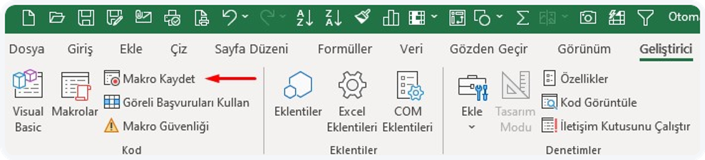
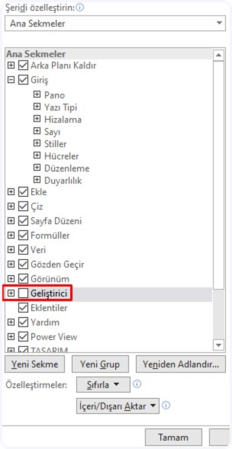
If you don’t have this menu in the Ribbon, you can add it like this:
File ‣ Options ‣ Customize the Ribbon ‣ Developer ‣ OK.


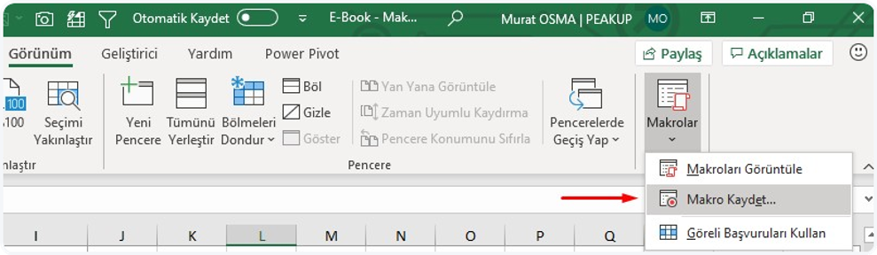
2- Through the View Menu


3- Through the StatusBar


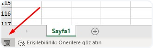
You can active the Record Macro feature by using the method you want.
Now I will tell you about how to activate it. But just read it, we will practice it together later.

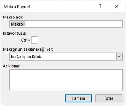
When your press Record Macro, this screen will pop up.
You can give a name in the Macro1 box about what you will do.
For example: if you will use it to filter, you can write filter and then press the OK button.
The moment we press it, the record will start, and it will record and codify each action in the background. When you are done, you need to Stop Recording. You can click Stop Recording in the same place.


Now, let’s see how easy it is with an example.

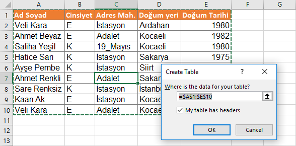
We all convert out data into a table. I mean, we have titles in the first row and data under those titles, right? And we filter many times in that table during the day. What do we do when we filter? We click the filter arrows in the field (column) to be filtered and select the data in the window that pops open or look it up and click OK and the table is filtered by the data we want.

We spend time even on this simple filter and lose extra time for nothing. Open the filter all the time, select, click OK. And when we are looking for another data, open the filter again, select and then click OK over and over again.

But only if we had an empty cell that we would use to filter and we could just click Enter or click the button to filter, wouldn’t that be way simpler and quicker?

This will save you time just for one action you will be executing in a day. But, imagine speeding up all your actions this way.


IN WHICH CASES CAN YOU RUN THE CODE YOU HAVE WRITTEN?

When you:

  • Select,
  • Righ-click,
  • Double-click a cell.
  • Enter data into the cell,
  • Open the page,
  • Open the file,
  • Close the file,
  • Click a button,
  • Press a key in your keyboard

etc. you can run the codes you have written.


Now, let’s execute this action with an applied example.

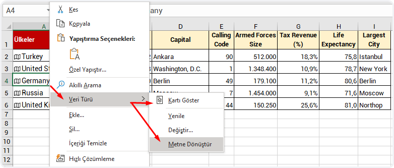
We have a file like in the image, you can try things out on that file and then practice on your own files.

Download the file here.

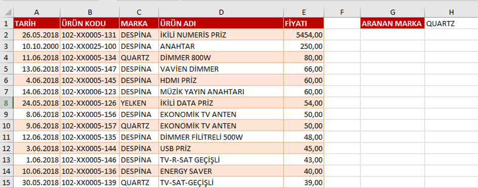
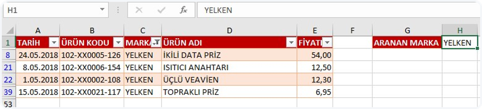
We want the data of a Brand to be filtered when we write that Brand’s name into the H1 cell in this file. When we write QUARTZ into the cell, the QUARTZ will be filtered in the Brand field. When we write YELKEN, YELKEN will be filtered. Thus, we will be using that cell as a filter box.


We will take the action in just a bit.

But before, you need to know this. There are fields to write codes depending on the running methods we have stated under the In Which Cases Can You Run the Code You Have Written? title.


These fields are:

  • Module – (Codes create with Record Macro or manually are stored here.)
  • Code Window of the Page (Code running actions of the related page are stored here.)
  • General Code Window of the Book (Actions that would affect the whole book are stored here.)

Since we want to filter when we enter a data into a cell in the page, we will paste the ready-made codes we have obtained with Record Macro to the Code Window of the Page. When data is entered to the cell, Change will be triggered and filter will be applied.


Don’t forget that you can use the Record Macro for all your tasks.


Let’s say that the steps to be taken will always be:

  • Click Record Macro
  • Manually do the action you want
  • Stop Recording

Codes will be prepared in the background.


WHERE CAN YOU ACCESS THESE CODES?


There are multiple ways to do something in Excel, just like in life. You can access these codes in a few different ways.

  1. By choosing View Macros where we chose Record Macro.

2. By pressing the Alt + F8 keys and accessing the window below with a shortcut.


3. By pressing the Alt + F11 keys and accessing the VBE window directly.

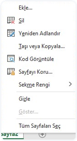
4. By choosing View Code after right-clicking the sheet tab.


Alriighht! Now that we have learnt enough, let’s take the action.

If you have already downloaded the file I have sent you, click Record Macro. Name your Macro, for example: Filter, and then click OK to start recording.

Choose any cell in our table and choose Filter in the Data menu.
Note: If you hover on the Filter a bit, it will give you the shortcut if there is. You can activate the filter with that shortcut as well.


And then unmark all in the Brand field and choose YELKEN, and then click OK.

Since we basically want to get the code of filtering, we have executed the action and we are done.

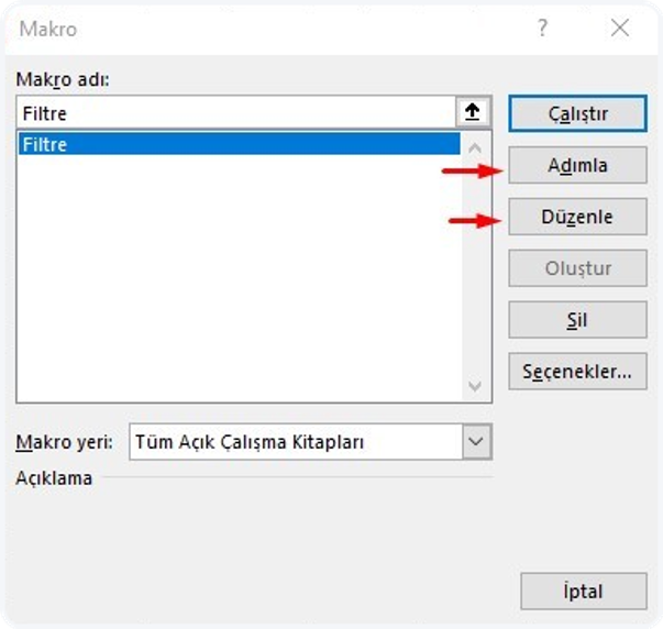
Now click Stop Recording to stop recording. Click View Macros.
The Macro List window will pop up and the Filter macro will be selected on it.
You can press the Edit button and view the codes in the Module1.

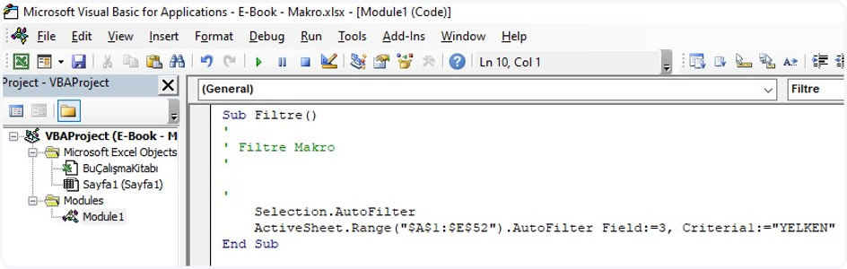
The codes that have been created will look like the image below.
The green rows that start with an apostrophe are comment rows, they don’t affect the codes, they are just for the explanation.
Note: You can delete the Selection.AutoFilter row. The row under it does the real job.


As you can see, we have easily obtained the codes of filtering.

Here is another information: You can assign the codes that start with Sub in the Module like above, and then run the macro by pressing the button. You can try this method if you please.

I will show how to filter the moment data is entered into the cell -which is a faster method. So, please keep reading.

Yes… we have obtained the codes.
Now there is only making the criteria dynamic so that it filters whatever we write into the H1 cell instead of “YELKEN” which was stated as the criterion in codes and running it when data is entered to the cell.


We will make a simple edit for this. Here is the code row that filters:

ActiveSheet.Range(“$A$1:$E$52″).AutoFilter Field:=3, Criteria1:=”YELKEN”


If you write the cell address like below where “YELKEN” is written in the code, you can use that cell as a filtering box dynamically.
ActiveSheet.Range(“$A$1:$E$52”).AutoFilter Field:=3, Criteria1:=Range(“H1”).Value


We have made the criteria dynamic. Now, let’s run this code depending on the data in the cell.
We have mentioned that we were going to write this code into the Change action of the Code Window of the Page since we want it to run when a data in the page changes.


So, what do we need to do now?


Right-click the tab and access the code window of the related page by choosing View Code. It will look like the image below at first.
Choose Worksheet in General.

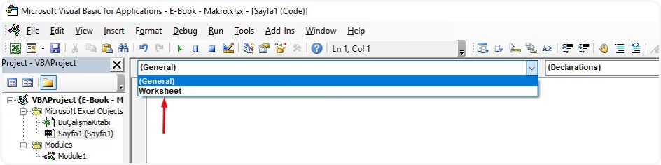
Page actions that you can use will be uploaded to the Declarations field, choose the Change action there.

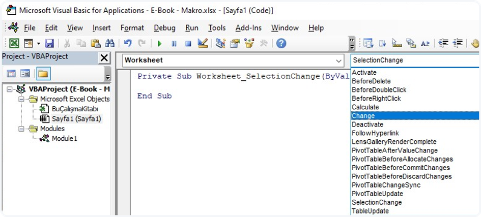
Related action will be added to the window.
Write the name of the macro we have created as Call Filter in that action.
Since the Selection_Change is unnecessary now, you can delete it.

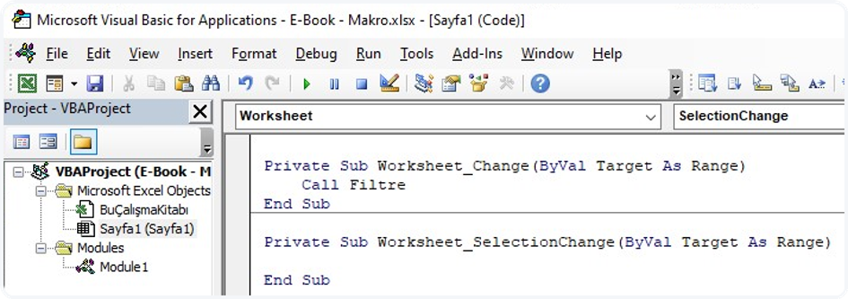
When a data is entered/changed in your page, the Filter macro will run.
At this point we might come across some difficulties. We have left our code as data entry in a cell, not in a certain cell. Even if we make a change in a cell other than H1, filtering will be done. Thus, after every action we take in the page, the filter will be applied.

It would make more sense to adjust is as run only a change is done in the H1 cell.
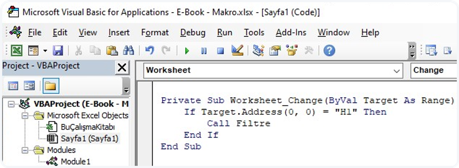
And if we accept this as the last touch to make the code run in a more stable way, we can settle the matter by adding a little condition.

That last touch will be this condition: If Target.Address(0, 0) = “H1” Then

Explanation: We complete our code by saying If the address of the cell into which data was entered is H1

You will see the result in the page like this. Whatever you write into H1, that name will be filtered in the Brand field.

Here is a little tip: if you write yel* into the cell and press Enter or add & “*”  to the end of the code, the cell will filter without you writing the full name of the brand. For example: if you write yel and press enter, it will list all the records that start with yel.

ActiveSheet.Range(“$A$1:$E$52”).AutoFilter Field:=3, Criteria1:=Range(“H1”).Value & “*”


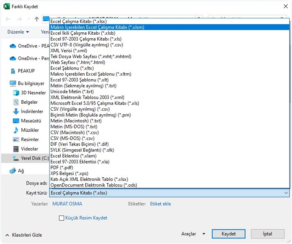
After everything is done and it is time to save the file, you need to save the file as Excel Macro-Enabled Workbook. (The Save As shortcut is F12.)


Congratulations! 👍🏻

You have just gained your first coding (creating a macro) experience.

These are very fun subjects, apart from also being very useful. I am sure the you will want more as you keep learning.
This article was for making you realize that you can get your tasks done quicker by codifying the actions you execute on Excel all the time.

You can access the last version of the file here.


Don’t forget that we can help you climb the success ladder in Excel with the Excel & VBA (Macro) Training and Consultancy Services as PEAKUP.

You can share this post to help many people get informed and get Excel Training to use Excel more efficiently and productively. 👍🏻

GEOGRAPHY LINKED DATA TYPE

GEOGRAPHY DATA TYPE

There were always data types in Excel. But they were traditional data types like text and number. Stocks and Geography data types are unique because they are accepted as linked data types. Linked data types have a connection to an online data source. For now, linked data types are only Stocks and Geography. Microsoft plans to share more linked data types in the future with the feedback from the clients. We will be sharing the new linked data types here.

Office 365 users can access a lot of data of countries by clicking their names only. You will see the Geography linked data type in the data Types group of the Data menu. This features allows us to get and list a lot of indicators like flags, capitals, currencies, data ratios, populations, military power, president, average life time of the countries through http://data.worldbank.org/. It is possible to access more detailed information of countries with the link I gave you, and you can even download this data in the Excel, Csv and Xml format and use them in your reports.


It is enough to write the country name in the A column one under another and choose the Geography type.


DATA CART

First, we wrote the names of 5 countries and chose the Geography data type.
After the country name in the cell is turned into the Geography data type, an icon is seen in the cell.
Click the icon to view the cart. Cart shows a list of areas and related values.
There might be a lot of areas that you can view and work with depending on the data. If you click the icon next to the country name, you will see that you can get the flag of that country and a lot more information.


When you select a country in a cell, an option list called Add Data pops up next to it.
When you choose the information you want to get from that list, that information will be listed quickly next to it.


You can list a lot of information about the country or countries you select next to one other and turn them into a table like below. If you want, you can indicate the data you want to get for a country and then drag it down to list the data of all countries in the indicated area.


You can write =A2. to call the data in the related areas from the defined names with a formula.


When you right-click the countries, you can see the Show Cart option within Data Type in the menu. (Ctrl + Shift + F5)  You can turn off the feature by converting the data into Text. You can cancel the Geography data type whenever you want like converting the tables into a range.


I hope this helps you.👍🏻
You can share this article with your friends and make it reach out to many people. Don’t forget: The more information is shared, the more valuable it gets.

HAVE YOU EVER SORTED WITH A FORMULA?

THE SORT FUNCTION


Hello everyone,

No doubt that one of the most frequently used functions in Excel is the Sort function.
This feature has 2 constants: A-Z and Z-A i.e. Ascending and Descending Sort.
We sort our data by certain field in pretty much all tables.
Have you ever tried to get this sorting action done with a formula?


WHAT DOES IT DO

You can easily sort columns or rows by the sort order you want in a different field from your mail table with the SORT function that is one of the dynamic array functions that are recently released after Office 365 . 


SYNTAX

=SORT(array,[sort_index],[sort_order],[by_col])

There are 4 arguments in the function.
The first one is required, the next 3 arguments are optional.

Now, let’s take a look at what these arguments mean, i.e. what the function wants from us and what we will give it.

Argument Description
array

Required

The range, or array to sort
[sort_index]

Optional

A number indicating the row or column to sort by
[sort_order]

Optional

A number indicating the desired sort order; 1 for ascending order (default), -1 for descending order
[by_col]

Optional

A logical value indicating the desired sort direction; FALSE to sort by row (default), TRUE to sort by column


USE OF THE FUNCTION

  • Choose the fields you want from your table and state by which column and order you will sort.
  • When you choose a field for the array argument only, the data is sort based on the Ascending order.
  • If multiple columns are selected in the array argument, the column by which the sorting will be done is chosen.
  • You can choose the Descending order in the sort_order argument if you want. If you don’ choose it, the sort is always Ascending.
  • In the by_col argument, you can sort by column i.e. from left to right. If not chosen, the sorting will always be from top to bottom.


Let’s have an example and see what happens when we choose the array argument only.


Now, let’s choose multiple columns and state the sort_index argument as well.


Since we didn’t use the sort_order argument in the formula below, prices are sorted from the lower to the higher. Now, let’s use the sort_order argument in the same function and see our data sorted from the higher to the lower.


Lastly, let’s sort the data from left to right and now from top to bottom.

We will be talking about the other New Dynamic Array functions in our next articles.
And then we will be able to get things done way easier by using these new functions together. LONG LIVE THE NEW DYNAMIC ARRAY FUNCTIONS!

See you in other articles, bye. 🙋🏻‍♂️
You can share this article and help a lot of people get informed as well. 👍🏻

FILTER: NEW GENERATION FUNCTION

THE FILTER FUNCTION

Hello everybody,

In this article, will talk about the abilities of the FILTER function that is one of the New Dynamic Array functions. As you know, new changes have been coming into our lives with the Office 365. We can tell from the new Office apps updates and fixes published in the Office Insider Fast channel that Microsoft cares about developing Excel -its one of the strongest weapons- and that has focused on this product with Teams.


I mentioned in the XLOOKUP article that I was going to talk about the FILTER function details in its own article. Now, it is this function’s turn.


WHAT DOES IT DO?

Imagine creating Filters in one field or more. You can list all the record quickly without filtering the rest of the data on the screen with the FILTER function. For example: List me all the Murats in the A column. As you know, the VLOOKUP function gives us one result and brings the first data it finds, unfortunately doesn’t bring the others. The FILTER function brings us all the records. Now we can list the data as a whole with this function without using macros of writing array formulas. The use of the function is quite simple, keep reading for the details. 👍🏻


SYNTAX

=FILTER(array; include; [if_empty])

There are 3 arguments in the function.
The first 2 are required and the last one is optional.

Now let’s take a look at what these arguments mean, i.e. what the function wants from us and what we will give it.

array

Required

The array, or range to filter
include

Required

A Boolean array whose height or width is the same as the array
[if_empty]

Optional

The value to return i


USE OF THE FUNCTION

First, let’s list the data based on one criterion.
Let’s list based on FİRMA(COMPANY) and all the records of that company. Let’s choose bring the data of the company we choose from the FİRMA SEÇ(CHOOSE COMPANY) cell and if you like, let’s send a message like “No Record” if no data is found. For this, when you write no record into the [if_empty] argument; the text will be written into the cell if a data will not be returned.


USING MULTIPLE DYNAMIC CRITERIA

Into the insert argument of the function, we can list the results as a whole if there is data that match the criteria you’ve stated in multiple fields. For example, let’s have two criteria and list the data that match these criteria in the COMPANY and PRODUCT fields. For this, we write each of our criteria into parenthesis and add * (star/cross) in between the criteria.


We will be talking about the other New Dynamic Array functions in our next articles.
And then we will be able to get things done way easier by using these new functions together. I can’t help but wish that these formulas have had come out 15 years ago. 😀 LONG LIVE THE NEW DYNAMIC ARRAY FUNCTIONS!

See you in other articles, bye. 🙋🏻‍♂️
You can share this article and help a lot of people get informed as well. 👍🏻

SORT DATA WITH THE SORTBY FUNCTION

THE SORTBY FUNCTION

Hello everybody,

There are functions about sorting among the newly released dynamic array functions. They are:

  • SORT
  • SORTBY

We will be talking about the SORTBY function in this article.


WHAT DOES IT DO

With the SORTBY function that is one one the recently release dynamic array functions after Office 365, you can sort your table based on multiple columns/rows and sort order you want in a field without touching your table. Imagine suing the Sort feature we use a lot in Excel through the Custom Sort window. If we want to sort by multiple fields, we choose a column there and use one of the A to Z or Z to A options in the Order field and then choose the other field and choose the sorting order again. Thus, our table is sorted by the columns/rows and order we chose. Now we can do all this with one single function.


SYNAX

=SORTBY(array, by_array1, [sort_order1], [by_array2, sort_order2],…) 

There are 3 arguments in the function.
The first two are required, the others are optional.

Now let’s take a look at what these arguments mean, i.e. what the function wants from us and what we will give it.

array

Required

The array or range to sort
by_array1

Required

The array or range to sort on
[sort_order1]

Optional

The order to use for sorting. 1 for ascending, -1 for descending. Default is ascendi


USE OF THE FUNCTION

  • the data range to be listed in the array argument.
  • the data range by which the sorting will be done based on which column/row first in the by_array1 argument.
  • the sort order is chosen in the sort_order1 argument. If it is not stated, the A to Z order is accepted.
  • you can continue by choosing a data range first and then sort order in the next optional array and orders.
  • you have to state at least one column/row in the by_array1 argument.


Let’s give an example and see what happens when only the optional arguments are chosen.


Now, let’s make the sort_order argument -1 and thus sort by Z to A .


SORT BY MULTIPLE FIELDS

We have sorted by one column and order so far. Now it is time to sort by multiple fields and orders. 😉 Let’s sort the Marka(Brand) field A to Z and then sort the Fiyat(Price) field Z to A and then change the sorting order of the Fiyat(Price) field and see the result.


SORT FROM LEFT TO RIGHT IN A HORIZONTAL TABLE

If you wish, you can sort the data in the field you’ve stated as an array by the stated array or order from left to right in a horizontal table. The important thing is to state the array to be returned, field to be sorted and the sorting order. The table will be sorted by the criteria you stated, doesn’t matter if it is vertical or horizontal.


We will be talking about the other New Dynamic Array functions in our next articles.
And then we will be able to get things done way easier by using these new functions together. LONG LIVE THE NEW DYNAMIC ARRAY FUNCTIONS!

See you in other articles, bye. 🙋🏻‍♂️
You can share this article and help a lot of people get informed as well. 👍🏻

GET RID OF DUPLICATE RECORDS WITH THE UNIQUE FUNCTION

THE UNIQUE FUNCTION


Hello everybody,

In this article I will be talking about one of the The Dynamic Array Functions -the UNIQUE function. Before this function, we had to write a long nested formula and even an array formula in order to list the unique data in one or multiple columns. But now we can list the unique data in the field you want with a single and very simple function.


WHAT DOES IT DO

The UNIQUE function allows you to create from the data in the stated field. Use this function to return a list of unique values in a list or range.  When you press Enter, the results can be displayed in a contiguous range with a suitable size.


SYNTAX

=UNIQUE(array; [by_col]; [exactly_once])

There are 3 arguments in the function.
The first one is required, the other two are optional.

Now let’s take a look at what these arguments mean, i.e. what the function wants from us and what we will give it.

Argument Description
array

Required

The range or array from which to return unique rows or columns
[by_col]

Optional

The by_col argument is a logical value indicating how to compare.

TRUE will compare columns against each other and return the unique columns

FALSE (or omitted) will compare rows against each other and return the unique rows

[exactly_once]

Optional

The exactly_once argument is a logical value that will return rows or columns that occur exactly once in the range or array. This is the database concept of unique.

TRUE will return all distinct rows or columns that occur exactly once from the range or array

FALSE (or omitted) will return all distinct rows or columns from the range or array

USE OF THE FUNCTION

We use this function to list the unique data in one column or multiple columns. For example, if we don’t know a formula to list the data in a row; we had to copy that column to a blank column and choose Remove Duplicates or we could list the Unique records only with the Advanced Filter. After writing this function, it will be enough to state the range from which we want the unique data.

You will see how easy it is one you watch the GIF below.

We have listed the unique data in the range we have stated by entering the first argument. Now let’s see what kind of results it returns with the other arguments.

The second arguments that is optional is the [by_col] argument.
TRUE and FALSE options are offered to us in this argument.
TRUE: Returns the unique columns.
FALSE: Returns the unique rows.

You can choose the FALSE option for the by_col argument if you want to get the unique data in any field.

UNIQUE / DUPLICATE DATA

The last argument [exactly_once] offers use two options concerning the data to be returned.
TRUE: Returns the data that is displayed only once. (Lists the ones that have been written only once, doesn’t take the ones written multiple times into consideration). FALSE: Returns all the different elements (Lists the unique ones in the range we choose).

We can choose the TRUE option if we want the data to be listed to be unique data only, and the FALSE option if we want the different data only.

Here is an example for that.


LONG LIVE THE NEW DYNAMIC ARRAY FUNCTIONS!


See you in other articles, bye. 🙋🏻‍♂️

You can share this post and help a lot of people get informed as well.👍🏻